Shadow tomography dari state Greenberger-Horne-Zeilinger

Perkiraan penggunaan: Kurang dari 10 detik pada prosesor Heron r2 (CATATAN: Ini hanya perkiraan. Waktu eksekusi kamu mungkin berbeda.)

Hasil pembelajaran

• Bagaimana shadow tomography membangun classical shadow dari sebuah state kuantum dan mengapa ia membutuhkan pengukuran yang jauh lebih sedikit secara eksponensial daripada tomografi state penuh

• Cara mengimplementasikan shadow tomography Pauli lokal memakai Qiskit untuk mengestimasi magnetisasi satu qubit, korelator dua titik, dan matriks densitas tereduksi dua qubit

• Cara memakai qiskit-paulice untuk deteksi error beroverhead rendah memakai spacetime code pada eksperimen hardware skala besar

Prasyarat

• Pengukuran

• Tomografi state kuantum

• Deteksi error memakai spacetime code

Latar belakang

Tomografi state kuantum penuh pada sistem $N$-qubit membutuhkan pengukuran yang jumlahnya eksponensial untuk mengestimasi semua $4^N -1$ parameter independen dari matriks densitas. Untuk sistem 50 qubit, misalnya, proses ini membutuhkan sekitar $10^{30}$ shot, yang lebih dari satu miliar kali jumlah bintang di alam semesta teramati. Shadow tomography [1] adalah protokol informasi kuantum yang membangun “classical shadow” dari state kuantum, yang darinya observabel target dapat diestimasi dengan jumlah shot yang berskala logaritmik terhadap jumlah observabel dan tidak bergantung pada ukuran sistem $N$, sehingga relevan di banyak bidang komputasi kuantum, termasuk estimasi energi, perhitungan entropi entanglement dan fungsi korelasi, estimasi kernel dalam machine learning kuantum, dan lainnya.

Tutorial ini menunjukkan cara memakai shadow tomography untuk mengestimasi observabel lokal, seperti magnetisasi satu qubit $\langle Z_i \rangle$ untuk qubit $i$, fungsi korelasi dua titik $\langle Z_i Z_j\rangle$, dan matriks densitas tereduksi dua qubit (2-RDM), dari state Greenberger-Horne-Zeilinger (GHZ) yang sangat entangled. Tutorial ini pertama-tama mengilustrasikan alur kerja shadow tomography skala kecil pada state GHZ 10 qubit memakai simulasi statevector. Lalu ia menunjukkan demonstrasi 100 qubit pada hardware kuantum sungguhan.

Protokol shadow tomography

Protokol shadow tomography memiliki langkah-langkah berikut:

1. Terapkan unitari acak $U$, yang diambil dari sebuah ensemble unitari, ke state kuantum awal.
2. Ukur hasilnya dalam basis komputasi, sehingga diperoleh bitstring $\ket{b}$.
3. Simpan snapshot klasik, $\hat{\rho} = \mathcal{M}^{-1}(U^{\dagger}\ket{b}\bra{b}U)$, dengan $\mathcal{M}^{-1}$ adalah invers dari kanal pengukuran $\mathcal{M}(\rho)=\mathbb{E}[U^{\dagger}\ket{b}\bra{b}U]$.
4. Ulangi proses ini sebanyak $T$ kali, di mana kumpulan $T$ snapshot $\{\hat{\rho}_t\}$ membentuk classical shadow $S(\rho, T)$.
5. Estimasi observabel $o$ dari operator $O$ sebagai $\frac{1}{T}\sum_{t=1}^{T}\text{Tr}(O\hat{\rho}_t)$.

Varian shadow tomography

Pilihan ensemble unitari, yaitu basis, pada langkah 1 protokol memengaruhi kompleksitas sampel, varians estimasi, dan kelengkapan informasi dari suatu shadow tomography. Banyak grup ensemble telah dipertimbangkan dalam literatur, masing-masing dengan trade-off antara kompleksitas dan efisiensi estimasi observabel. Properti varian yang paling umum dipakai dirangkum dalam tabel berikut, meskipun daftar ini tidak lengkap.

Varian	Ensemble	Kompleksitas sampel	Kedalaman circuit	Observabel yang cocok
Pauli lokal [1]	Pauli satu qubit $\{X, Y, Z\}$	$\mathcal{O}(3^k\text{log}M/\varepsilon^2)$	1	lokal/few-body
Clifford global [1]	Clifford $N$-qubit	$\mathcal{O}(\text{Tr}(O^2)\text{log}M/\varepsilon^2)$	$\mathcal{O}(N\text{log}N)$	rank rendah, fidelitas
Gaussian fermionik [2], [3]	circuit matchgate	$\mathcal{O}(\binom{\mu}{k}\frac{1}{\varepsilon^2})$	$\mathcal{O}(N^2)$	fermionik
shallow shadows [4], [5]	circuit berkedalaman rendah	$\mathcal{O}(k2^k\text{log}M/\varepsilon^2)$	$\mathcal{O}(\text{log}N)$	non-lokal (ramah hardware)

Istilah yang dipakai dalam tabel didefinisikan sebagai berikut:

• "kompleksitas sampel" mengacu pada jumlah pengukuran yang dibutuhkan untuk suatu varian shadow tomography.

• "kedalaman circuit" menggambarkan seberapa mahal pengukuran untuk diimplementasikan pada hardware kuantum.

• $N$ adalah jumlah qubit.

• $k$ adalah lokalitas observabel (misalnya, $\langle Z_i \rangle$ punya $k=1$ dan $\langle Z_i Z_j\rangle$ punya $k=2$).

• $M$ adalah jumlah observabel yang diestimasi secara bersamaan.

• $\varepsilon$ adalah toleransi error aditif.

• $\mu$ adalah jumlah fermion.

Meskipun ensemble Pauli lokal paling ramah hardware, ia menanggung penalti kompleksitas sampel $3^k$, sehingga kurang cocok untuk estimasi properti non-lokal. Secara lebih umum, batas kompleksitas sampel local-shadow berskala $4^k$, membaik menjadi $3^k$ pada kasus khusus observabel hasil kali tensor.

Sebaliknya, meskipun ensemble Clifford global bisa dipakai untuk mengestimasi observabel non-lokal, kedalaman circuit-nya kurang menguntungkan. Shadow Gaussian fermionik berguna dalam simulasi fisika many-body, kimia, dan material, tetapi membutuhkan circuit matchgate, yang mungkin membawa overhead signifikan pada perangkat berbasis gate serbaguna.

Shallow shadows punya kedalaman circuit di antara Pauli lokal dan Clifford global, sehingga menjadi varian yang sangat menjanjikan untuk implementasi praktis, meskipun masih ada beberapa pertanyaan terbuka mengenai kedalaman circuit optimal untuk suatu observabel.

Seiring terus berkembangnya frontier riset shadow tomography, beberapa masalah paling relevan yang perlu ditangani mencakup pemilihan ensemble pengukuran yang optimal untuk himpunan observabel target, perbaikan batas kompleksitas sampel, dan perluasan protokol ke observabel yang berevolusi terhadap waktu. Meskipun demikian, shadow tomography tetap menjadi salah satu alur kerja terdepan untuk mengekstrak informasi klasik maksimal dari sebuah state kuantum dengan jumlah pengukuran minimum, sehingga ideal untuk mengkarakterisasi state kuantum pada skala di mana tomografi penuh maupun simulasi klasik tidak mungkin dilakukan.

Ensemble Pauli lokal

Tutorial ini memakai basis Pauli acak, yaitu gate Clifford satu qubit, untuk mengumpulkan shadow dan mengestimasi properti state GHZ. Perhatikan bahwa pengukuran Pauli adalah pilihan yang bagus untuk mengestimasi observabel lokal (seperti densitas spin, fungsi korelasi lokal, dan densitas probabilitas posisi), tetapi tidak untuk observabel global (seperti energi total, momentum, dan muatan).

Di sini, basis Pauli acak $\{X, Y, Z\}$ dipilih secara independen untuk setiap qubit dan rotasi satu qubit yang sesuai diterapkan, diikuti pengukuran:

$$\begin{equation} U = U_0 \otimes U_1 \otimes \cdots \otimes U_{n-1}, U_q \in \{I, H, S^{\dagger}H\} \end{equation} \tag{1}$$

Untuk ensemble ini, invers dari kanal pengukuran adalah:

$$\begin{equation} \hat{\rho}_q=3U_q^{\dagger}\ket{b_q}\bra{b_q}U_q - I \end{equation} \tag{2}$$

Faktor $3$ berasal dari perataan atas tiga basis Pauli, yang menghasilkan kanal depolarisasi dengan parameter $\frac{1}{3}$. Estimator penuhnya kemudian terfaktorisasi sebagai hasil kali estimator satu qubit. Seperti ditunjukkan dalam tabel, untuk $M$ observabel, masing-masing berlokalitas $k$, jumlah shadow Pauli yang dibutuhkan untuk mengestimasi semua observabel hingga error aditif $\varepsilon$ dengan probabilitas tinggi adalah $\mathcal{O}(\frac{3^k\text{log}(M)}{\varepsilon^2})$. Ukuran sistem tidak memengaruhi biaya pengukuran selama observabelnya tetap lokal, sehingga observabel yang jumlahnya eksponensial dapat diestimasi sekaligus dengan biaya yang hanya logaritmik.

Median of means

Rata-rata biasa atas $T$ snapshot mengurangi varians dari estimasi satu-shot suatu observabel sebesar $\frac{1}{T}$, tetapi sensitif terhadap outlier. Median of means dapat dipakai untuk mengatasinya. Prosesnya meliputi:

• Membagi $T$ snapshot menjadi $K$ grup berukuran sama
• Menghitung rata-rata dalam setiap grup
• Mengembalikan median dari rata-rata grup

Tutorial ini melakukan shadow tomography Pauli lokal untuk mengestimasi properti state GHZ, pertama memakai contoh simulasi 10 qubit lalu mendemonstrasikan eksperimen hardware 100 qubit.

Persyaratan

Sebelum memulai tutorial ini, pastikan kamu sudah menginstal yang berikut:

• Qiskit SDK v2.0 atau lebih baru, dengan dukungan visualisasi

• IBM Quantum Compute v0.28 atau lebih baru (pip install qiskit-ibm-runtime)

• Qiskit Paulice (pip install qiskit-paulice)

Penyiapan

# Added by doQumentation — installs the packages this notebook needs if they are missing
import importlib.util

_needed = {"matplotlib": "matplotlib", "numpy": "numpy", "qiskit": "qiskit", "qiskit_ibm_runtime": "qiskit-ibm-runtime", "qiskit_paulice": "qiskit-paulice"}
_missing = [pip for module, pip in _needed.items()
            if importlib.util.find_spec(module) is None]
# One at a time, so a package that fails to install does not block the others
for _pip in _missing:
    %pip install -q {_pip}
if not _missing:
    print("\u2713 All required packages are installed")

import numpy as np
import matplotlib.pyplot as plt
from collections import deque, defaultdict
from qiskit import QuantumCircuit, ClassicalRegister
from qiskit.quantum_info import (
    Statevector,
    partial_trace,
    Operator,
    Pauli,
    SparsePauliOp,
)
from qiskit.transpiler import generate_preset_pass_manager
from qiskit_ibm_runtime import QiskitRuntimeService
from qiskit_ibm_runtime import SamplerV2 as Sampler
from qiskit_paulice.layout import get_low_overhead_ancillas

seed = 42  # for reproducibility
rng = np.random.default_rng(seed)

Fungsi helper berikut dipakai oleh contoh hardware skala besar di bagian akhir tutorial:

• bad_cz, bad_readout, bad_coherence — Mengquery data kalibrasi backend untuk mengidentifikasi gate, qubit, dan edge yang melebihi ambang error atau koherensi, sehingga bisa dikecualikan dari layout circuit.

• parallel_ghz — Membangun circuit GHZ dengan ukuran tertentu memakai breadth-first search pada coupling map, menyebar layer CNOT secara paralel untuk meminimalkan kedalaman circuit.

• weighted_coverage, active_wires, z_trace_backward — Menghitung seberapa besar permukaan error circuit GHZ yang dilindungi oleh sekumpulan pemeriksaan paritas spacetime tertentu, memakai teknik propagasi mundur dari [6].

• add_measurements — Menambahkan pengukuran qubit GHZ dan qubit pemeriksaan ke register klasik terpisah sehingga bisa dipostseleksi secara independen.

• build_shadow_circuits — Menghasilkan satu circuit per basis Pauli acak dengan menambahkan rotasi satu qubit yang sesuai sebelum pengukuran.

• parse_hw_results_w_checks — Membongkar output Sampler menjadi triplet (ghz_bits, check_bits, bases), satu per shot.

• adapt_to_flat_bits, estimate_zz_nn_hw — Memetakan bit register GHZ kembali ke ruang indeks perangkat penuh dan menghitung estimasi median-of-means $\langle Z_i Z_{i+1}\rangle$.

def bad_cz(target, threshold: float = 0.01) -> list:
    "Return edges whose CZ error exceeds threshold."
    edges = []
    for edge in backend.target.build_coupling_map().get_edges():
        if (edge[1], edge[0]) not in edges:
            edges.append(edge)
    cz_errors = {edge: target["cz"][edge].error for edge in edges}
    worst = sorted(cz_errors.items(), key=lambda x: x[1], reverse=True)
    return [list(edge) for edge, error in worst if error > threshold]

def bad_readout(target, threshold: float = 0.01) -> list:
    "Return nodes whose measurement error exceeds threshold."
    meas_errors = {
        node: target["measure"][(node,)].error
        for node in range(backend.num_qubits)
    }
    worst = sorted(meas_errors.items(), key=lambda x: x[1], reverse=True)
    return [node for node, error in worst if error > threshold]

def bad_coherence(target, threshold: float = 60) -> list:
    "Return nodes whose T2 value is below threshold."
    t2s = {
        node: (target.qubit_properties[node].t2 or 0) * 1e6
        for node in range(backend.num_qubits)
    }
    return [
        node
        for node, val in sorted(t2s.items(), key=lambda x: x[1])
        if val < threshold
    ]

def parallel_ghz(
    root: int, num_qubits: int, backend, bad_edges: list, skip: list
) -> tuple:
    "Build a GHZ circuit of size num_qubits using BFS from root, one neighbor per layer."
    edges = [
        e
        for e in [list(e) for e in backend.coupling_map.get_edges()]
        if e not in bad_edges
        and [e[1], e[0]] not in bad_edges
        and e[0] not in skip
        and e[1] not in skip
    ]
    adj = defaultdict(list)
    for u, v in edges:
        adj[u].append(v)
        adj[v].append(u)

    qc = QuantumCircuit(backend.num_qubits)
    visited = [root]
    queue = deque([root])
    explored = defaultdict(set)
    layers = []
    qc.h(root)

    while queue and len(visited) < num_qubits:
        layer = []
        for node in list(queue):
            queue.popleft()
            unvisited = [
                nb
                for nb in adj[node]
                if nb not in visited and nb not in explored[node]
            ]
            if unvisited:
                nb = unvisited[0]
                visited.append(nb)
                queue.append(node)
                queue.append(nb)
                explored[node].add(nb)
                layer.append((node, nb))
                if len(visited) == num_qubits:
                    break
        if layer:
            layers.append(layer)
        else:
            break

    for layer in layers:
        for q1, q2 in layer:
            qc.cx(q1, q2)
        qc.barrier()

    return qc, visited, layers

def weighted_coverage(
    layers: list, parities: list, w_idle: float = 0.2, w_gate: float = 0.8
) -> float:
    "Compute weighted fraction of wires covered by at least one parity check."
    wires = active_wires(layers)
    covered_by_any = {n_layer: set() for n_layer in range(len(layers))}
    for parity in parities:
        for n_layer, qs in z_trace_backward(layers, parity).items():
            covered_by_any[n_layer] |= qs
    covered_weight = total_weight = 0
    for n_layer in range(len(layers)):
        idle = wires[n_layer]["idle"]
        gate = wires[n_layer]["gate"]
        total_weight += w_idle * len(idle) + w_gate * len(gate)
        covered_weight += w_idle * len(
            covered_by_any[n_layer] & idle
        ) + w_gate * len(covered_by_any[n_layer] & gate)
    return covered_weight / total_weight if total_weight > 0 else 0

def active_wires(layers: list) -> dict:
    """
    Returns per-layer dict with two sets:
    - 'idle': activated wires that are idle in this layer
    - 'gate': activated wires that are control/target of a CNOT at this layer
    """
    first_activation = {}
    for n_layer, layer in enumerate(layers):
        for c, t in layer:
            first_activation.setdefault(c, n_layer)
            first_activation.setdefault(t, n_layer)
    result = {}
    for n_layer in range(len(layers)):
        active = {
            q
            for q, n_layer0 in first_activation.items()
            if n_layer >= n_layer0
        }
        gate = {q for c, t in layers[n_layer] for q in (c, t)}
        result[n_layer] = {"idle": active - gate, "gate": gate}
    return result

def z_trace_backward(layers: list, initial_Zs: list) -> dict:
    """
    Backward propagate Zs with parity cancellation.
    Returns {layer: set of qubits with odd parity Z at that layer}.
    """
    wires = active_wires(layers)
    support = set(initial_Zs)
    trace = {}
    for n_layer in range(len(layers) - 1, -1, -1):
        active = wires[n_layer]["idle"] | wires[n_layer]["gate"]
        trace[n_layer] = support & active
        new_support = set()
        for q in support:
            hit = False
            for c, t in layers[n_layer]:
                if q == t:
                    new_support ^= {t, c}
                    hit = True
                    break
                elif q == c:
                    new_support ^= {c}
                    hit = True
                    break
            if not hit:
                new_support ^= {q}
        support = new_support
    return trace

def add_measurements(
    qc: QuantumCircuit, ghz_qubits: list, checks: list
) -> QuantumCircuit:
    "Add GHZ and check qubit measurements into separate classical registers."
    c1 = ClassicalRegister(len(ghz_qubits), "c1")
    qc.add_register(c1)
    for q, c in zip(ghz_qubits, c1):
        qc.measure(q, c)
    c2 = ClassicalRegister(len(checks), "c2")
    qc.add_register(c2)
    for q, c in zip(checks, c2):
        qc.measure(q, c)
    return qc

def build_shadow_circuits(
    base_circuit: QuantumCircuit,
    n_measure: int,
    ghz_qubits: list,
    checks: list,
) -> tuple:
    "Build n_measure circuits by appending random Pauli basis rotations to each GHZ qubit."
    n = base_circuit.num_qubits
    all_bases = rng.integers(0, 3, size=(n_measure, n))
    circuits = []
    for m in range(n_measure):
        qc = base_circuit.copy()
        qc.barrier()
        for q in ghz_qubits:
            b = all_bases[m, q]
            if b == 1:
                qc.h(q)
            elif b == 2:
                qc.sdg(q)
                qc.h(q)
        add_measurements(qc, ghz_qubits, checks)
        circuits.append(qc)
    return circuits, all_bases

def parse_hw_results_w_checks(
    result, bases: np.ndarray, ghz_qubits: list, checks: list
) -> list:
    "Parse hardware bitstrings into (ghz_bits, check_bits, bases) triples."
    snapshots = []
    n_ghz = len(ghz_qubits)
    n_checks = len(checks)
    for t, pub_result in enumerate(result):
        ghz_strings = (
            pub_result.data.c1.get_bitstrings()
        )  # one entry per shot
        chk_strings = pub_result.data.c2.get_bitstrings()
        for ghz_bitstring, check_bitstring in zip(ghz_strings, chk_strings):
            ghz_bits = [
                int(ghz_bitstring[n_ghz - 1 - i]) for i in range(n_ghz)
            ]
            check_bits = [
                int(check_bitstring[n_checks - 1 - i])
                for i in range(n_checks)
            ]
            snapshots.append((ghz_bits, check_bits, bases[t]))
    return snapshots

def adapt_to_flat_bits(
    ghz_bits: list, ghz_qubits: list, n_total: int
) -> list:
    "Map GHZ-register bits back to a full n_total-length bit vector."
    bits = [0] * n_total
    for i, q in enumerate(ghz_qubits):
        bits[q] = ghz_bits[i]
    return bits

def estimate_zz_nn_hw(
    snapshots: list, ghz_qubits: list, n_total: int, n_groups: int
) -> np.ndarray:
    "Estimate <ZiZi+1> for each neighboring GHZ qubit pair from flat-bit snapshots."
    pairs = list(zip(ghz_qubits[:-1], ghz_qubits[1:]))
    all_est = np.column_stack(
        [
            snapshot_estimate(
                ["Z" if q in pair else "I" for q in range(n_total)], snapshots
            )
            for pair in pairs
        ]
    )
    return mom(all_est, n_groups).real

Contoh simulator skala kecil

Pertama, siapkan state GHZ 10 qubit memakai simulasi statevector dan estimasi propertinya memakai shadow Pauli lokal. State GHZ adalah state kuantum yang maksimal entangled dengan tiga qubit atau lebih, yang menjadi tolok ukur untuk entanglement multipartit. State ini merupakan blok bangunan umum untuk protokol komunikasi kuantum dan kriptografi. Selain itu, circuit GHZ punya properti analitik yang diketahui sepenuhnya, sehingga ideal untuk verifikasi dalam tutorial ini.

Langkah 1: Petakan input klasik ke masalah kuantum

Siapkan state GHZ 10 qubit yang ideal.

def ghz_statevector(num_qubits):
    qc = QuantumCircuit(num_qubits)
    qc.h(0)
    for q in range(num_qubits - 1):
        qc.cx(q, q + 1)
    return Statevector(qc)

num_qubits = 10  # number of qubits
psi = ghz_statevector(num_qubits)
psi.seed(seed)
print(
    f"{num_qubits}-qubit GHZ state ready (norm = {np.linalg.norm(psi):.6f})"
)

10-qubit GHZ state ready (norm = 1.000000)

Langkah 2: Optimalkan untuk eksekusi di hardware kuantum

Selanjutnya, definisikan fungsi yang mengumpulkan snapshot shadow dengan merotasi state GHZ ke basis Pauli acak. Ini meniru apa yang dilakukan primitif Sampler pada hardware dalam contoh skala besar.

def basis_circuit(b):
    """0 -> Z basis (I), 1 -> X basis (H), 2 -> Y basis (Sdg;H)."""
    qc = QuantumCircuit(1)
    if b == 1:
        qc.h(0)
    elif b == 2:
        qc.sdg(0)
        qc.h(0)
    # b == 0: Z basis, no rotation
    return qc

_basis = {
    b: basis_circuit(b) for b in (0, 1, 2)
}  # built once, shared with the estimator's _U

def collect_shadow_snapshots(psi, n_snapshots, num_qubits):
    snapshots = []
    for _ in range(n_snapshots):
        bases = rng.integers(0, 3, size=num_qubits)
        rot = QuantumCircuit(num_qubits)
        for q, b in enumerate(bases):
            rot.compose(_basis[b], qubits=[q], inplace=True)
        evolved = psi.evolve(rot)
        evolved.seed(int(rng.integers(0, 2**31)))
        bitstr = next(
            iter(evolved.sample_counts(shots=1))
        )  # Born rule internal
        bits = [int(x) for x in bitstr[::-1]]  # little-endian -> qubit
        snapshots.append((bits, bases))
    return snapshots

Langkah 3: Eksekusi memakai primitif Qiskit

Untuk simulasi ini, pakai statevector secara langsung.

n_snapshots = 5000  # number of shadow snapshots
n_groups = 20  # groups/batches for median-of-means

snapshots = collect_shadow_snapshots(psi, n_snapshots, num_qubits)
print(f"Collected {n_snapshots} snapshots.")

Collected 5000 snapshots.

Langkah 4: Pasca-proses dan kembalikan hasil dalam format klasik yang diinginkan

Definisikan shadow estimator dan median-of-means (MOM) estimator untuk basis pengukuran acak yang dipakai buat mengumpulkan snapshot shadow. Pakai fungsi-fungsi ini untuk memperkirakan properti state GHZ, termasuk magnetisasi single-qubit, korelator dua-qubit, dan RDM dua-qubit, dari hasil pengukuran yang terkumpul. Lalu bandingkan estimasinya dengan nilai eksak.

_U = {
    b: Operator(basis_circuit(b)) for b in (0, 1, 2)
}  # rotation Uᵢ per basis
_P = {p: Operator(Pauli(p)) for p in "IXYZ"}  # single-qubit Paulis

def shadow_estimator(P, b, bit):  # P is a label char, e.g. "X"
    UPU = _U[b] @ _P[P] @ _U[b].adjoint()  # Uᵢ P Uᵢ†
    return (3 * UPU.data[bit, bit] - np.trace(_P[P].data)).real

def mom(estimates: np.ndarray, n_groups: int) -> np.ndarray:
    "Median-of-means outlier suppression."
    T = len(estimates)
    spg = T // n_groups  # shots per group
    trimmed = estimates[
        : spg * n_groups
    ]  # drop any leftover shots that don't cleanly fit into a group
    groups = trimmed.reshape(n_groups, spg, *estimates.shape[1:])
    means = groups.mean(axis=1)  # take the mean of each group
    return np.median(means.real, axis=0) + 1j * np.median(
        means.imag, axis=0
    )  # take the median of means for real and imaginary parts separately

def snapshot_estimate(
    pauli_string, snapshots
):  # full-width label, len == num_qubits
    out = np.empty(len(snapshots), dtype=complex)
    for t, (bits, bases) in enumerate(snapshots):
        e = 1.0 + 0j
        for q, P in enumerate(pauli_string):
            e *= shadow_estimator(P, bases[q], bits[q])
        out[t] = e
    return out

Z_est = np.column_stack(
    [
        snapshot_estimate(
            ["Z" if q == i else "I" for q in range(num_qubits)], snapshots
        )
        for i in range(num_qubits)
    ]
)
Z_vals = mom(Z_est, n_groups).real

ZZ_est = np.column_stack(
    [
        snapshot_estimate(
            ["Z" if q in (i, i + 1) else "I" for q in range(num_qubits)],
            snapshots,
        )
        for i in range(num_qubits - 1)
    ]
)
ZZ_nn = mom(ZZ_est, n_groups).real

ZZ_full = np.zeros((n_snapshots, num_qubits, num_qubits), dtype=complex)
for i in range(num_qubits):
    ZZ_full[:, i, i] = 1.0  # diagonal is always 1
    for j in range(i + 1, num_qubits):
        col = snapshot_estimate(
            ["Z" if q in (i, j) else "I" for q in range(num_qubits)],
            snapshots,
        )
        ZZ_full[:, i, j] = col
        ZZ_full[:, j, i] = col  # symmetric
ZZ_mat = mom(ZZ_full, n_groups).real

# 2-qubit reduced density matrix (RDM) for pair (qi, qj)
# the elementwise complex median (real/imag split) for the RDM coefficients generalizes the scalar median in Ref.[1]
qi, qj = 0, num_qubits - 1
terms = []
for a in "IXYZ":
    for b in "IXYZ":
        label = "".join({qi: a, qj: b}.get(q, "I") for q in range(num_qubits))
        c = mom(snapshot_estimate(label, snapshots).reshape(-1, 1), n_groups)[
            0
        ]
        terms.append((b + a, c / 4))
rho_shadow = SparsePauliOp.from_list(terms).to_matrix()

traced_out = [q for q in range(num_qubits) if q not in (qi, qj)]
rho_exact = partial_trace(
    psi, traced_out
).data  # diag(0.5, 0, 0, 0.5) for GHZ

print(f"{'Observable':<22} {'Estimated':>12} {'Ideal':>8} {'Max error':>12}")
print("-" * 57)
print(
    f"{'<Zi> (all qubits)':<22} {'-':>12} {'0':>8} {np.max(np.abs(Z_vals)):>12.4f}"
)
print(
    f"{'<ZiZi+1> mean':<22} {np.mean(ZZ_nn):>12.4f} {'1':>8} {np.max(np.abs(ZZ_nn - 1)):>12.4f}"
)
print(
    f"{'2-RDM Frobenius err':<22} {'-':>12} {'0':>8} {np.linalg.norm(rho_shadow - rho_exact):>12.4f}"
)

Observable                Estimated    Ideal    Max error
---------------------------------------------------------
<Zi> (all qubits)                 -        0       0.0540
<ZiZi+1> mean                1.0040        1       0.1520
2-RDM Frobenius err               -        0       0.1080

Visualisasikan hasilnya

Plot pertama menunjukkan nilai magnetisasi single-qubit hasil estimasi untuk tiap qubit. Plot kedua menunjukkan distribusi nilai korelator dua titik hasil estimasi untuk semua pasangan qubit. Plot terakhir menunjukkan besaran entri matriks densitas tereduksi dua-qubit. Jumlah snapshot yang dipakai cukup besar untuk ukuran sistem ini, jadi hasilnya dekat dengan nilai eksak.

fig, axes = plt.subplots(
    1, 3, figsize=(14, 4), gridspec_kw={"width_ratios": [1, 1, 1]}
)

z_exact = psi.expectation_value(
    SparsePauliOp.from_sparse_list([("Z", [0], 1.0)], num_qubits)
).real  # 0.0
zz_exact = psi.expectation_value(
    SparsePauliOp.from_sparse_list([("ZZ", [0, 1], 1.0)], num_qubits)
).real  # 1.0

# <Zi>
axes[0].bar(range(num_qubits), Z_vals, color="#4a90d9", alpha=0.85)
axes[0].axhline(0, color="black", lw=0.8)
axes[0].set_ylim(-0.5, 0.5)
axes[0].set_title(r"$\langle Z_i \rangle$ (ideal = %0.2f)" % z_exact)
axes[0].set_xlabel("Qubit index")
axes[0].grid(axis="y", alpha=0.3)

# <ZiZj>
im = axes[1].imshow(ZZ_mat, vmin=-1, vmax=1, cmap="magma")
plt.colorbar(im, ax=axes[1])
axes[1].set_title(r"$\langle Z_i Z_j \rangle$ (ideal = %0.2f)" % zz_exact)
axes[1].set_xlabel("Qubit j")
axes[1].set_ylabel("Qubit i")

# 2-RDM magnitude
im2 = axes[2].imshow(np.abs(rho_shadow), vmin=0, vmax=0.5, cmap="Blues")
plt.colorbar(im2, ax=axes[2])
axes[2].set_title(r"$|\rho_2|$ for qubits (0, N-1)")
axes[2].set_xticks(range(4))
axes[2].set_yticks(range(4))
axes[2].set_xticklabels(["00", "01", "10", "11"])
axes[2].set_yticklabels(["00", "01", "10", "11"])

[Text(0, 0, '00'), Text(0, 1, '01'), Text(0, 2, '10'), Text(0, 3, '11')]

Menilai penskalaan shot

Di tutorial ini, 5.000 snapshot dipakai untuk memperkirakan observabel. Penskalaan shot pada shadow tomography dinilai dengan memplot rata-rata error dari salah satu fungsi hasil estimasi terhadap berbagai anggaran shot. Error pada korelator dua-qubit menurun sebesar $1/\sqrt{T}$, sesuai dengan konvergensi statistik standar untuk mean estimator. Keunggulan shadow tomography adalah faktor konstanta di depan $1/\sqrt{T}$ tidak membesar seiring bertambahnya jumlah qubit untuk observabel lokal, seperti yang dibahas di tutorial ini.

shot_counts = [100, 250, 500, 1000, 2000, 5000, 10000]
errors = []

for N_test in shot_counts:
    snaps = collect_shadow_snapshots(psi, N_test, num_qubits)
    zz_vals = []
    for i in range(num_qubits - 1):
        ests = []
        for bits, bases in snaps:
            e = 1.0 + 0j
            for q in range(num_qubits):
                op = "Z" if q in (i, i + 1) else "I"
                e *= shadow_estimator(op, bases[q], bits[q])
            ests.append(e.real)
        zz_vals.append(np.mean(ests))
    errors.append(float(np.mean(np.abs(np.array(zz_vals) - 1.0))))
    print(f"T={N_test:5d} error = {errors[-1]:.4f}")

fig, ax = plt.subplots(figsize=(6, 4))
T_arr = np.array(shot_counts, dtype=float)
ax.loglog(T_arr, errors, "o-", color="#4a90d9", lw=2, label="Shadow estimate")
ax.loglog(
    T_arr,
    errors[0] * np.sqrt(shot_counts[0] / T_arr),
    "k--",
    alpha=0.5,
    label=r"$1/\sqrt{T}$ reference",
)
ax.set_xlabel("Shots T")
ax.set_ylabel(r"Mean $|\langle Z_i Z_{i+1} \rangle - 1|$")
ax.set_title(f"Convergence for {num_qubits}-qubit GHZ")
ax.legend()
plt.tight_layout()
plt.show()

T=  100 error = 0.1856
T=  250 error = 0.1613
T=  500 error = 0.1027
T= 1000 error = 0.0827
T= 2000 error = 0.0513
T= 5000 error = 0.0311
T=10000 error = 0.0162

Contoh hardware skala besar

Simulasi sebelumnya mengonfirmasi bahwa local Pauli shadow tomography memulihkan observabel yang benar pada statevector tanpa noise. Menjalankan protokol yang sama dengan 100 qubit di hardware sungguhan menimbulkan dua tantangan yang tidak muncul di simulasi: error Gate dan readout menumpuk di sepanjang Circuit GHZ yang dalam, dan menemukan layout qubit yang optimal butuh pencarian di graf coupling perangkat, bukan memilih layout secara manual.

Untuk mengatasi tantangan pertama, gunakan deteksi error dengan overhead rendah memakai spacetime codes [6]. Sejumlah kecil qubit ancilla yang bersebelahan dengan pohon GHZ dipakai sebagai parity check. Tiap ancilla di-entangle dengan dua tetangganya di GHZ sebelum diukur, sehingga satu bit-flip error pada salah satu tetangga membalik hasil ancilla dari 0 menjadi 1. Snapshot yang punya ancilla pemeriksa bernilai 1 dibuang, menyisakan subset yang lebih bersih untuk memperkirakan $\langle Z_i Z_{i+1}\rangle$.

Tantangan kedua diatasi dengan mencari berbagai kandidat layout pohon GHZ lalu memilih yang memaksimalkan cakupan parity-check, yaitu fraksi wire Circuit yang dipantau oleh setidaknya satu pemeriksa, dengan kenaikan kedalaman Circuit yang masih dapat diterima.

Langkah 1-4 (dijalankan dalam satu blok kode)

Alur kerja empat langkah yang sama sekarang diterapkan ke state GHZ 100-qubit di hardware kuantum sungguhan, dengan menambahkan dua fitur khusus hardware yang tidak muncul di simulasi:

• Langkah 1 mengkarakterisasi noise Backend (error Gate, error readout, dan waktu T2) supaya qubit dan edge yang tidak andal dikeluarkan dari layout Circuit.

• Langkah 2 mencari berbagai layout pohon GHZ untuk menemukan yang memaksimalkan cakupan parity-check dalam kedalaman Circuit yang masih dapat diterima, menggantikan rantai sederhana yang dipakai di simulasi.

• Langkah 3 membangun Circuit shadow (satu per basis Pauli acak), men-transpile-nya ke Gate native hardware, dan mengirimkannya ke primitive Sampler dengan shots=8 (tiap Circuit menghasilkan delapan bitstring independen).

• Langkah 4 melakukan postselect pada snapshot yang semua qubit pemeriksanya bernilai 0 (tidak ada error terdeteksi), lalu memperkirakan $\langle Z_i Z_{i+1}\rangle$ dengan dan tanpa postselection tersebut untuk menunjukkan peningkatan dari deteksi error.

# ── Step 1: Map classical inputs to a quantum problem ─────────────────────────
service = QiskitRuntimeService()
backend = service.least_busy(
    operational=True, simulator=False, min_num_qubits=133
)
coupling_map = backend.target.build_coupling_map()
n_total = backend.num_qubits

thresh_cz, thresh_meas, thresh_t2 = 0.025, 0.15, 10
bad_edges = bad_cz(backend.target, threshold=thresh_cz)
bad_nodes_readout = bad_readout(backend.target, threshold=thresh_meas)
dead_qubits = bad_readout(backend.target, threshold=0.4)
bad_nodes = list(
    set(bad_nodes_readout)
    | set(bad_coherence(backend.target, threshold=thresh_t2))
)

# ── Step 2: Optimize for quantum hardware execution ───────────────────────────
# Search over starting qubits and random node-skip sets to find the GHZ layout
# with the best parity-check coverage within an acceptable circuit depth.
ghz_size = 100
max_skips, shuffles, max_depth_increase = 10, 200, 10
w_idle, w_gate = 0.2, 0.8

# Find the root that yields the shallowest GHZ — exclude bad_nodes from the start
best_root = None
base_depth = float("inf")
for root in range(backend.num_qubits):
    if root in bad_nodes:
        continue
    qc, ghz_qubits, _ = parallel_ghz(
        root, ghz_size, backend, bad_edges, bad_nodes
    )
    if len(ghz_qubits) != ghz_size:
        continue
    depth = qc.depth(lambda x: x.operation.num_qubits == 2)
    if depth < base_depth:
        best_root, base_depth = root, depth
if best_root is None:
    raise Exception(
        "No qualifying GHZ root layout found. Relax error thresholds."
    )

qc, ghz_qubits, layers = parallel_ghz(
    best_root, ghz_size, backend, bad_edges, bad_nodes
)

degree_two_nodes = [
    i
    for i in ghz_qubits
    if all(n in ghz_qubits for n in coupling_map.neighbors(i))
    and len(coupling_map.neighbors(i)) >= 2
]

best_covered_fraction = -1
best_qc = best_checks = best_parities = best_layers = best_ghz_qubits = None

for num_skips in range(max_skips):
    for _ in range(shuffles):
        skip_trial = list(
            rng.choice(degree_two_nodes, num_skips, replace=False)
        )
        qc, ghz_qubits, layers = parallel_ghz(
            best_root, ghz_size, backend, bad_edges, skip_trial + bad_nodes
        )
        if len(ghz_qubits) != ghz_size:
            continue
        depth = qc.depth(lambda x: x.operation.num_qubits == 2)
        checks, parities = [], []
        for ancilla, neighbors in get_low_overhead_ancillas(
            coupling_map, ghz_qubits
        ).items():
            if ancilla in dead_qubits:
                continue
            good_neighbors = [
                n
                for n in neighbors
                if [ancilla, n] not in bad_edges
                and [n, ancilla] not in bad_edges
            ]
            if len(good_neighbors) < 2:
                continue
            checks.append(ancilla)
            parities.append((good_neighbors[0], good_neighbors[1]))
            qc.cx(good_neighbors[0], ancilla)
            qc.cx(good_neighbors[1], ancilla)
        covered_fraction = weighted_coverage(
            layers=layers, parities=parities, w_idle=w_idle, w_gate=w_gate
        )
        if (
            covered_fraction > best_covered_fraction
            and depth <= base_depth + max_depth_increase
        ):
            best_covered_fraction = covered_fraction
            (
                best_qc,
                best_ghz_qubits,
                best_checks,
                best_parities,
                best_layers,
            ) = qc, ghz_qubits, checks, parities, layers

qc, ghz_qubits, checks, parities, layers = (
    best_qc,
    best_ghz_qubits,
    best_checks,
    best_parities,
    best_layers,
)
if len(ghz_qubits) != ghz_size:
    raise Exception("No GHZ found. Relax error thresholds.")

print(f"GHZ qubits: {ghz_qubits} ({len(ghz_qubits)})")
print(f"Check qubits: {checks} ({len(checks)})")
print(
    "Covered fraction (no idle): ",
    weighted_coverage(
        layers=layers, parities=parities, w_idle=0.0, w_gate=1.0
    ),
)

# ── Step 3: Execute using Qiskit primitives ───────────────────────────────────
# Build one shadow circuit per random Pauli basis, each repeated for shots_per_basis
# independent bitstrings. Transpile to hardware-native gates, then submit using the
# Sampler primitive. Each circuit yields shots_per_basis snapshots in that basis.
n_hw = 1000
shots_per_basis = 8  # multiple shots per basis circuit
shadow_circs, hw_bases = build_shadow_circuits(qc, n_hw, ghz_qubits, checks)
sampler = Sampler(backend)
sampler.options.environment.job_tags = ["TUT_STGHZS"]
pm = generate_preset_pass_manager(optimization_level=1, backend=backend)
isa_circuit = pm.run(shadow_circs)
job = sampler.run(isa_circuit, shots=shots_per_basis)
result = job.result()

# ── Step 4: Post-process and return result in desired classical format ─────────
# Filter snapshots whose check qubits all read 0 (no detected error), then
# estimate <ZiZi+1> with and without the error-detection postselection.
snapshots_hw = parse_hw_results_w_checks(result, hw_bases, ghz_qubits, checks)
snapshots_kept = [
    (ghz_bits, check_bits, bases)
    for (ghz_bits, check_bits, bases) in snapshots_hw
    if all(b == 0 for b in check_bits)
]
snapshots_kept_adapted = [
    (adapt_to_flat_bits(ghz_bits, ghz_qubits, n_total), bases)
    for (ghz_bits, check_bits, bases) in snapshots_kept
]
snapshots_hw_adapted = [
    (adapt_to_flat_bits(ghz_bits, ghz_qubits, n_total), bases)
    for (ghz_bits, check_bits, bases) in snapshots_hw
]

print("Shadow snapshots collected:", len(snapshots_hw))
print("Shadow snapshots kept post error-detection:", len(snapshots_kept))

n_groups = min(5, len(snapshots_kept))  # groups for median-of-means
ZZ_hw = estimate_zz_nn_hw(snapshots_hw_adapted, ghz_qubits, n_total, n_groups)
ZZ_kept = estimate_zz_nn_hw(
    snapshots_kept_adapted, ghz_qubits, n_total, n_groups
)

# Plot <ZiZi+1> before and after error detection
fig, axes = plt.subplots(1, 2, figsize=(13, 4))

axes[0].plot(ZZ_hw, "o-", color="#e05c5c", markersize=4)
axes[0].axhline(1.0, color="gray", ls="--", alpha=0.7, label="Ideal")
axes[0].set_ylim(-0.6, 3.0)
axes[0].set_title(r"$\langle Z_i Z_{i+1} \rangle$ (without error detection)")
axes[0].set_xlabel("GHZ qubit pair")
axes[0].legend()
axes[0].grid(alpha=0.3)

axes[1].plot(ZZ_kept, "o-", color="#e05c5c", markersize=4)
axes[1].axhline(1.0, color="gray", ls="--", alpha=0.7, label="Ideal")
axes[1].set_ylim(-0.6, 3.0)
axes[1].set_title(r"$\langle Z_i Z_{i+1} \rangle$ (with error detection)")
axes[1].set_xlabel("GHZ qubit pair")
axes[1].legend()
axes[1].grid(alpha=0.3)

plt.tight_layout()
plt.show()

print("Before detection: <ZiZi+1>= ", float(np.average(ZZ_hw)))
print("After detection: <ZiZi+1>= ", float(np.average(ZZ_kept)))

GHZ qubits: [57, 47, 67, 46, 66, 48, 45, 65, 49, 44, 64, 38, 43, 77, 29, 42, 85, 28, 56, 41, 84, 30, 27, 36, 86, 31, 21, 87, 32, 20, 88, 33, 22, 97, 89, 34, 23, 107, 78, 39, 35, 16, 106, 90, 69, 53, 19, 24, 3, 108, 105, 91, 70, 52, 15, 25, 2, 109, 104, 92, 71, 54, 51, 14, 4, 1, 110, 103, 98, 93, 58, 55, 13, 5, 0, 118, 96, 72, 59, 12, 6, 129, 102, 73, 11, 7, 128, 101, 74, 10, 8, 127, 100, 9, 126, 116, 125, 121, 124, 120] (100)
Check qubits: [68, 37, 50, 63, 83, 17, 26, 18, 117, 111, 75] (11)
Covered fraction (no idle):  0.5454545454545454
Shadow snapshots collected: 8000
Shadow snapshots kept post error-detection: 566

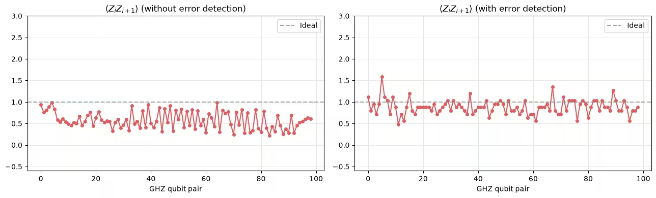
Before detection: <ZiZi+1>=  0.573749999999951
After detection: <ZiZi+1>=  0.8817377312951776

Menafsirkan hasil

Kedua plot menunjukkan $\langle Z_i Z_{i+1}\rangle$ hasil estimasi shadow tomography untuk setiap pasangan qubit bertetangga di rantai GHZ 100-qubit, sebelum dan sesudah postselection pada parity check.

Untuk state GHZ ideal, semua korelator tetangga terdekat bernilai $1$. Di hardware, noise menurunkan estimasi mentah dan menimbulkan sebaran antar qubit. Setelah deteksi error, snapshot yang mengandung setidaknya satu error terdeteksi dibuang, dan estimasi yang tersisa bergeser lebih dekat ke $1$ dengan varians lebih kecil, yang sesuai dengan state efektif yang lebih bersih.

Peningkatan setelah deteksi error sesuai dengan pemeriksa yang mendeteksi error sungguhan.

Langkah selanjutnya

Jelajahi sumber daya berikut untuk belajar lebih lanjut:

Rekomendasi

• General formulation of quantum information
• Low-overhead error detection using spacetime codes tutorial
• Qiskit Paulice add-on API documentation

Referensi

• [1] Huang, H. Y., Kueng, R., & Preskill, J. (2020). Predicting many properties of a quantum system from very few measurements. Nature Physics, 16, 1050–1057.

• [2] Zhao, A., Rubin, N. C., & Miyake, A. (2021). Fermionic partial tomography via classical shadows. Phys. Rev. Lett., 127, 110504.

• [3] Low, G. H. (2022). Classical shadows of fermions with particle number symmetry. arXiv:2208.08964.

• [4] Bertoni, C., Haferkamp, J., Hinsche, M. et al. (2024). Shallow Shadows: Expectation Estimation Using Low-Depth Random Clifford Circuits. Phys. Rev. Lett., 133, 020602.

• [5] Hu, H.-Y., Gu, A., Majumder, S. et al. (2025). Demonstration of robust and efficient quantum property learning with shallow shadows. Nature Communications, 16, 2943.

• [6] Martiel, S. & Javadi-Abhari, A. (2025). Low-overhead error detection with spacetime codes. arXiv:2504.15725. © IBM Corp. 2026