Deteksi error dengan overhead rendah menggunakan spacetime codes

Estimasi penggunaan: 4 menit pada prosesor Heron (ibm_kingston atau setara) (CATATAN: Ini hanya perkiraan. Runtime Anda mungkin bervariasi.)

Hasil pembelajaran

• Bagaimana spacetime Pauli checks mendeteksi error logis dalam circuit Clifford, dan bagaimana postselecting pada syndrome-nya meningkatkan fidelitas distribusi yang disampel.

• Cara menggunakan paket qiskit-paulice untuk menemukan dan menyisipkan check yang hardware-efficient secara otomatis dengan get_check_qubits, NoiseModel, dan add_pauli_checks.

• Cara mengestimasi fidelitas state stabilizer dengan menyampel stabilizer-nya dan melakukan postselect pada check syndrome.

• Cara menjalankan alur kerja deteksi error lengkap pada hardware IBM Quantum® dan membandingkan fidelitas noisy dan postselected.

Prasyarat

• Dasar-dasar hardware untuk komputasi kuantum skala utilitas.

• Formalisme Clifford dan stabilizer, termasuk bagaimana grup stabilizer mendeskripsikan state stabilizer murni.

Latar belakang

Low-overhead error detection with spacetime codes [1] oleh Simon Martiel dan Ali Javadi-Abhari memperkenalkan metode untuk mendeteksi error logis dalam circuit yang didominasi Clifford yang berada di antara koreksi error penuh dan mitigasi error yang lebih ringan. Ide ini dibangun berdasarkan coherent Pauli checks (CPC) dari Single-shot error mitigation by coherent Pauli checks [2] oleh van den Berg dan lainnya. Dalam kedua pendekatan tersebut, circuit "payload" Clifford di-entangle dengan qubit ancilla untuk memeriksa invarian tertentu. Mengukur ancilla menghasilkan syndrome yang melaporkan apakah error terdeteksi selama eksekusi. Hanya menyimpan sampel tanpa error yang terdeteksi meningkatkan fidelitas distribusi yang disampel, dengan biaya berupa laju postselection yang berkurang.

Perbedaan utama antara coherent Pauli checks dan spacetime checks adalah operator yang mereka ukur. Coherent Pauli checks mengukur operator yang terlokalisasi dalam waktu dan berbobot tinggi. Pada topologi qubit dengan konektivitas terbatas, seperti heavy hex, check tersebut membutuhkan banyak gate SWAP dan sering membuat circuit terlalu dalam untuk dijalankan secara praktis. Mengimplementasikan check sebagai spacetime codes justru mendistribusikan setiap check ke seluruh circuit payload dalam ruang dan waktu. Ini menghasilkan encoding yang hardware-efficient yang tetap efektif dalam mendeteksi error logis sambil menjaga overhead qubit dan kedalaman tetap rendah.

Apa yang dilakukan paket qiskit-paulice

Paket qiskit-paulice mengotomatiskan konstruksi check ini sehingga Anda tidak perlu membangunnya secara manual. Peran utamanya adalah menemukan dan menyisipkan spacetime Pauli checks yang valid pada lokasi-lokasi dalam circuit yang memaksimalkan deteksi error sambil meminimalkan overhead qubit. Sebuah check dikatakan valid ketika operatornya tidak mengubah aksi logis dari circuit payload, low-weight ketika menggunakan sedikit entangling gate, dan efektif ketika mendeteksi sebagian besar error, relatif terhadap noise yang diperkenalkan oleh check itu sendiri. Paket ini menilai kandidat check terhadap model noise dan mengomit yang terbaik ke dalam circuit. Tutorial ini menggunakan tiga metode API:

• get_check_qubits memeriksa coupling map backend dan mengembalikan pasangan qubit target dan ancilla. Sebuah check pada target_qubits[i] menggunakan ancilla_qubits[i].

• NoiseModel.from_backend membangun model noise kasar dari data benchmark backend. Model ini menilai kandidat check, sehingga model noise yang tepat dan dipelajari tidak diperlukan. Untuk model Pauli-Lindblad yang dipelajari, lihat NoiseModel.from_pauli_lindblad_maps.

• add_pauli_checks menemukan dan menyisipkan check ke dalam circuit. Ini mengembalikan urutan objek CheckedCircuit dengan jumlah check yang meningkat, dan setiap objek menyediakan get_postselection_method yang memetakan bitstring yang diukur ke vektor syndrome. Argumen cost memilih fungsi yang menilai suatu check (gamma, overhead sampling dari kanal noise invers yang di-postselect, atau LER, laju error logis). Argumen method memilih strategi pencarian (windowed, genetic, atau windowed_genetic). Tutorial ini menggunakan cost="gamma" dan method="windowed", yang bersama-sama memberikan pemilihan check yang deterministik dan dapat direproduksi.

Mengestimasi fidelitas dari sampling stabilizer

Untuk mengukur seberapa baik deteksi error bekerja, Anda dapat mengestimasi fidelitas state stabilizer $|\psi\rangle = U|0\rangle^{\otimes n}$ yang secara ideal disiapkan oleh circuit terhadap state noisy $\rho$ yang sebenarnya dihasilkan oleh hardware. Proyektor pada state stabilizer murni $|\psi\rangle$ sama dengan rata-rata seragam pada $2^n$ elemen dari grup stabilizer-nya $\mathcal{S}$:

$|\psi\rangle\langle\psi| = \frac{1}{2^n}\sum_{G \in \mathcal{S}} G.$

Mensubstitusikan ini ke dalam fidelitas memberikan fidelitas $\rho$ sebagai nilai ekspektasi rata-rata dari setiap stabilizer $G \in \mathcal{S}$ terhadap $\rho$:

$F = \mathrm{Tr}(\rho|\psi\rangle\langle\psi|) = \frac{1}{2^n} \sum_{G \in \mathcal{S}} \mathrm{Tr}(\rho G) = \frac{1}{2^n} \sum_{G \in \mathcal{S}} \langle G \rangle_\rho.$

Untuk masalah yang lebih besar, mengenumerasi semua $2^n$ stabilizer tidak layak, sehingga Anda dapat mengestimasi fidelitas dari sampel acak. Mengambil $M$ stabilizer $G_1, \ldots, G_M$ secara seragam acak dari $\mathcal{S}$ memberikan estimasi yang tidak bias:

$\hat F_M = \frac{1}{M} \sum_{i=1}^M \langle G_i \rangle_\rho.$

Karena circuit Clifford menyiapkan state stabilizer, Anda dapat mengestimasi fidelitasnya langsung dari nilai ekspektasi stabilizer yang disampel. Tutorial ini pertama-tama membahas alur kerja pada simulator dengan circuit kecil, kemudian menjalankan alur kerja yang sama pada hardware dengan circuit yang lebih besar dan lebih dalam. Seiring circuit menyertakan lebih banyak operasi non-Clifford, jumlah check yang valid menyusut dengan cepat, sehingga metode ini bekerja paling baik untuk circuit yang didominasi Clifford.

Persyaratan

Sebelum memulai tutorial ini, pastikan Anda telah menginstal hal berikut:

• Qiskit SDK v2.0 atau lebih baru, dengan dukungan visualisasi

• Qiskit Runtime v0.40 atau lebih baru (pip install qiskit-ibm-runtime)

• Qiskit Aer v0.17 atau lebih baru (pip install qiskit-aer)

• Qiskit Paulice (pip install qiskit-paulice)

• tqdm (pip install tqdm)

Persiapan

Impor library yang diperlukan dan definisikan fungsi helper yang tidak tersedia sebagai impor. Fungsi random_clifford_circuit membangun payload Clifford acak brickwork, find_check_layout menelusuri coupling map backend untuk menemukan jalur qubit ber-error rendah yang memiliki banyak ancilla yang tersedia, learned_noise_model mengubah output NoiseLearner menjadi model noise qiskit-paulice, append_basis_rotation merotasi circuit sehingga stabilizer diukur dalam basis komputasi, expectation menghitung nilai ekspektasi stabilizer dari counts yang disampel, dan cum_mean_sem melacak estimasi fidelitas yang berjalan.

# Added by doQumentation — required packages for this notebook
!pip install -q matplotlib numpy qiskit qiskit-aer qiskit-ibm-runtime qiskit-paulice tqdm

# Standard library imports
import random
import time

# External libraries
import matplotlib.pyplot as plt
import numpy as np
from tqdm import tqdm

# Qiskit
from qiskit import QuantumCircuit
from qiskit.quantum_info import Clifford, Pauli, PauliLindbladMap, PauliList
from qiskit.result import sampled_expectation_value
from qiskit.transpiler import generate_preset_pass_manager
from qiskit.visualization import plot_coupling_map

# Qiskit Aer
from qiskit_aer import AerSimulator
from qiskit_aer.noise import NoiseModel as AerNoiseModel
from qiskit_aer.noise import ReadoutError, depolarizing_error

# Qiskit IBM Runtime
from qiskit_ibm_runtime import NoiseLearner, QiskitRuntimeService
from qiskit_ibm_runtime import SamplerV2 as Sampler

# Qiskit Paulice
from qiskit_paulice import add_pauli_checks
from qiskit_paulice.layout import get_check_qubits
from qiskit_paulice.noise_models import NoiseModel

def random_clifford_circuit(
    num_qubits: int, depth: int, rng: np.random.Generator
) -> QuantumCircuit:
    """Brickwork random Clifford on `num_qubits`, with `depth` CZ layers."""
    qc = QuantumCircuit(num_qubits)
    qc.h(range(num_qubits))
    for d in range(depth):
        for i in range(d % 2, num_qubits - 1, 2):
            qc.cz(i, i + 1)
        for q in range(num_qubits):
            if rng.integers(0, 2):
                qc.sx(q)
            if rng.integers(0, 2):
                qc.s(q)
            if rng.integers(0, 2):
                qc.sx(q)
    return qc

def find_check_layout(
    backend,
    num_qubits: int,
    rng: np.random.Generator,
    num_trials: int = 200,
    max_gate_error: float = 0.03,
    max_readout_error: float = 0.2,
) -> list[int]:
    """Find a low-error path of `num_qubits` qubits with many available ancillas.

    Builds random self-avoiding walks on the coupling map, excluding the qubits
    and two-qubit gates whose reported errors exceed the thresholds, and keeps
    the path that offers the most target and ancilla pairs. Ties are broken by
    the lower average two-qubit gate error along the path.
    """
    target = backend.target
    gate_2q = next(
        name for name in ("cz", "ecr", "cx") if name in target.operation_names
    )

    # Collect per-edge gate errors and per-qubit readout errors
    edge_error = {}
    for qubits, props in target[gate_2q].items():
        edge = tuple(sorted(qubits))
        if props is not None and props.error is not None:
            edge_error[edge] = min(edge_error.get(edge, 1.0), props.error)
    readout_error = {
        qubit: target["measure"][(qubit,)].error
        for (qubit,) in target["measure"]
    }

    # Keep only the edges whose gate and readout errors are acceptable
    adjacency = {}
    for (q1, q2), error in edge_error.items():
        if (
            error <= max_gate_error
            and readout_error.get(q1, 1.0) <= max_readout_error
            and readout_error.get(q2, 1.0) <= max_readout_error
        ):
            adjacency.setdefault(q1, set()).add(q2)
            adjacency.setdefault(q2, set()).add(q1)

    # Random self-avoiding walks; keep the path with the most check pairs
    starts = sorted(adjacency)
    best_path = None
    best_score = (-1, float("inf"))
    for _ in range(num_trials):
        path = [starts[rng.integers(len(starts))]]
        while len(path) < num_qubits:
            options = sorted(adjacency[path[-1]] - set(path))
            if not options:
                break
            path.append(options[rng.integers(len(options))])
        if len(path) < num_qubits:
            continue
        num_pairs = len(get_check_qubits(backend.coupling_map, path)[0])
        mean_error = float(
            np.mean(
                [edge_error[tuple(sorted(e))] for e in zip(path, path[1:])]
            )
        )
        if num_pairs > best_score[0] or (
            num_pairs == best_score[0] and mean_error < best_score[1]
        ):
            best_path, best_score = path, (num_pairs, mean_error)

    if best_path is None:
        raise RuntimeError(
            "No connected low-error path found. Relax the error thresholds."
        )
    return best_path

def learned_noise_model(layer_errors, layout: list[int]) -> NoiseModel:
    """Build a `NoiseModel` from `NoiseLearner` results.

    `NoiseLearner` reports one `PauliLindbladError` per entangling layer, whose
    generators are indexed against that layer's own physical qubits, while
    `NoiseModel.from_pauli_lindblad_maps` expects `PauliLindbladMap`s indexed the
    way `NoiseModel.from_backend` indexes them: by position in `layout`. This
    translates between the two and drops generators that fall outside `layout`.
    """
    phys_to_virt = {phys: virt for virt, phys in enumerate(layout)}
    maps = []
    for layer in layer_errors:
        if layer.error is None:
            continue
        terms = []
        for pauli, rate in zip(
            layer.error.generators, layer.error.rates, strict=True
        ):
            label, indices = [], []
            for local, phys in enumerate(layer.qubits):
                x, z = bool(pauli.x[local]), bool(pauli.z[local])
                if not (x or z):
                    continue
                if phys not in phys_to_virt:
                    break  # generator reaches outside the layout, so skip it
                label.append("Y" if x and z else "X" if x else "Z")
                indices.append(phys_to_virt[phys])
            else:
                if label:
                    terms.append(
                        ("".join(label), tuple(indices), float(rate))
                    )
        # Each map needs a 2-qubit generator to define an entangling layer
        if any(len(t[1]) == 2 for t in terms):
            maps.append(
                PauliLindbladMap.from_sparse_list(
                    terms, num_qubits=len(layout)
                )
            )
    if not maps:
        raise RuntimeError(
            "No usable layer errors. Check that the learner ran on this layout."
        )
    return NoiseModel.from_pauli_lindblad_maps(maps)

def append_basis_rotation(
    circuit: QuantumCircuit, pauli: Pauli
) -> QuantumCircuit:
    """Strip measurements, append basis rotations for `pauli`, and re-measure."""
    out = circuit.remove_final_measurements(inplace=False)
    for q in range(pauli.num_qubits):
        if pauli.x[q]:
            if pauli.z[q]:
                out.sdg(q)
            out.h(q)
    out.measure_all()
    return out

def expectation(counts: dict, pauli: Pauli) -> float:
    """Expectation value of `pauli` from counts measured in the Z basis.

    Pads with identity on any qubits beyond the support of `pauli`, such as the
    check ancillas that appear in the postselected counts.
    """
    if not counts:
        return float("nan")
    n = pauli.num_qubits
    sign = -1 if int(pauli.phase) % 4 == 2 else 1
    total = len(next(iter(counts)))
    label = "".join(
        "Z" if q < n and (pauli.x[q] or pauli.z[q]) else "I"
        for q in range(total - 1, -1, -1)
    )
    return sign * sampled_expectation_value(counts, label)

def cum_mean_sem(values: np.ndarray):
    """Cumulative mean and standard error of the mean, ignoring NaNs."""
    valid = ~np.isnan(values)
    total = np.cumsum(np.where(valid, values, 0.0))
    total_sq = np.cumsum(np.where(valid, values**2, 0.0))
    count = np.maximum(np.cumsum(valid).astype(float), 1)
    mean = total / count
    sem = np.sqrt(np.maximum(total_sq / count - mean**2, 0) / count)
    return np.where(np.cumsum(valid) > 0, mean, np.nan), sem

Contoh simulator skala kecil

Bagian ini membahas alur kerja penuh pada simulator yang noisy. Ini menggunakan data benchmark backend untuk memilih layout qubit dan model noise, menemukan check secara otomatis, dan menggunakan postselection pada distribusi yang disampel untuk menunjukkan peningkatan fidelitas.

Langkah 1: Memetakan input klasik ke masalah kuantum

Circuit payload adalah circuit Clifford acak brickwork satu dimensi yang dangkal. Karena circuit ini Clifford, ia menyiapkan state stabilizer yang fidelitasnya dapat Anda estimasi langsung dari nilai ekspektasi stabilizer yang disampel. Mulailah dengan circuit yang dangkal sehingga check mudah divisualisasikan pada langkah berikutnya.

num_qubits = 12
depth = 4
seed = 1764
rng = np.random.default_rng(seed)
np.random.seed(seed)

circuit = random_clifford_circuit(num_qubits, depth, rng)
circuit.measure_all()
circuit.draw("mpl", fold=-1, scale=0.6)

Langkah 2: Mengoptimalkan untuk eksekusi hardware kuantum

Memetakan circuit ke hardware menentukan layout qubit fisik, model noise yang menilai kandidat check, dan check itu sendiri.

Pertama, pilih backend dan telusuri coupling map-nya untuk menemukan layout qubit satu dimensi dengan helper find_check_layout yang didefinisikan pada bagian Persiapan. Helper ini membangun random self-avoiding walk yang menghindari gate dan readout dengan error tertinggi, dan menyimpan jalur yang menawarkan pasangan target dan ancilla terbanyak. Karena pencarian membaca konektivitas dan data error dari backend itu sendiri, kode yang sama berjalan pada QPU IBM Quantum mana pun. Fungsi get_check_qubits kemudian mengembalikan pasangan target dan ancilla, di mana check pada target_qubits[i] menggunakan ancilla_qubits[i].

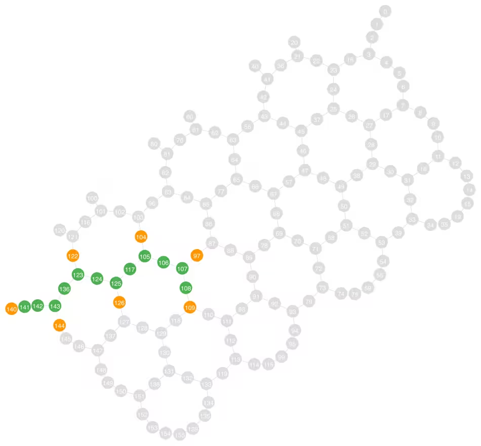
Pada graf coupling yang mengikuti, qubit hijau adalah qubit payload dan qubit oranye adalah ancilla yang mengimplementasikan check. Qubit dengan ancilla yang berdekatan digunakan sebagai qubit target untuk check.

service = QiskitRuntimeService()
backend = service.least_busy(operational=True, simulator=False)

print(f"Backend: {backend.name}")

# Search for a low-error path, then pair each target qubit with a neighboring ancilla
layout = find_check_layout(backend, num_qubits, rng)
target_qubits, ancilla_qubits = get_check_qubits(backend, layout)
num_checks = len(target_qubits)

print(f"Target qubits:  {target_qubits}")
print(f"Ancilla qubits: {ancilla_qubits}")
plot_coupling_map(
    num_qubits=backend.num_qubits,
    qubit_coordinates=getattr(
        backend.configuration(), "qubit_coordinates", None
    ),
    coupling_map=backend.configuration().coupling_map,
    figsize=(12, 12),
    qubit_color=[
        "#4CAF50"
        if i in set(layout)
        else "#FF9800"
        if i in set(ancilla_qubits)
        else "#DDDDDD"
        for i in backend.coupling_map.graph.node_indices()
    ],
    qubit_size=220,
    line_width=2,
    font_size=90,
)

Backend: ibm_boston
Target qubits:  [105, 107, 108, 123, 125, 141, 143]
Ancilla qubits: [104, 97, 109, 122, 126, 140, 144]

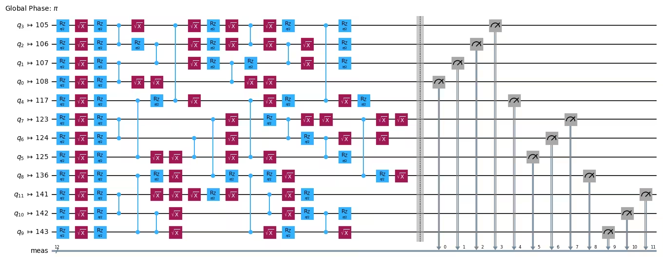
Dengan backend dan layout yang dipilih, transpile payload menjadi circuit instruction set architecture (ISA). Hanya perlu mengatur layout dan menerjemahkan gate ke dalam native gate set backend.

pm = generate_preset_pass_manager(
    optimization_level=0, backend=backend, initial_layout=layout
)
circuit_isa = pm.run(circuit)
circuit_isa.draw("mpl", fold=-1, scale=0.6)

Selanjutnya, modelkan bagaimana noise gate dan readout pada backend memengaruhi eksekusi. Model noise menentukan di mana dalam circuit sebuah check menangkap error paling banyak. Model yang lebih akurat meningkatkan deteksi, tetapi biasanya tidak perlu mempelajarinya dengan menyampel QPU. Model berikut menyimpulkan kanal depolarizing seragam untuk noise gate dan readout dari data benchmark qiskit-ibm-runtime.

noise_model = NoiseModel.from_backend(
    backend, layout, uniform_gate_noise=True
)
print(noise_model)

NoiseModel(gate_noise=0.001079865281450939, readout_noise=0.006001790364583333, idling_noise=None)

Sekarang tambahkan check ke circuit. Fungsi add_pauli_checks mengambil payload Clifford, daftar qubit target, dan model noise. Argumen ancilla_qubits memberi tahu fungsi ancilla fisik mana yang dipasangkan dengan setiap target. Check ditambahkan dalam urutan kemunculan qubit target, sehingga layout akhir dari circuit yang telah dicheck adalah layout + ancilla_qubits. Untuk menjalankan circuit output dengan lebih sedikit (i) check, layout akhir adalah layout + ancilla_qubits[:i].

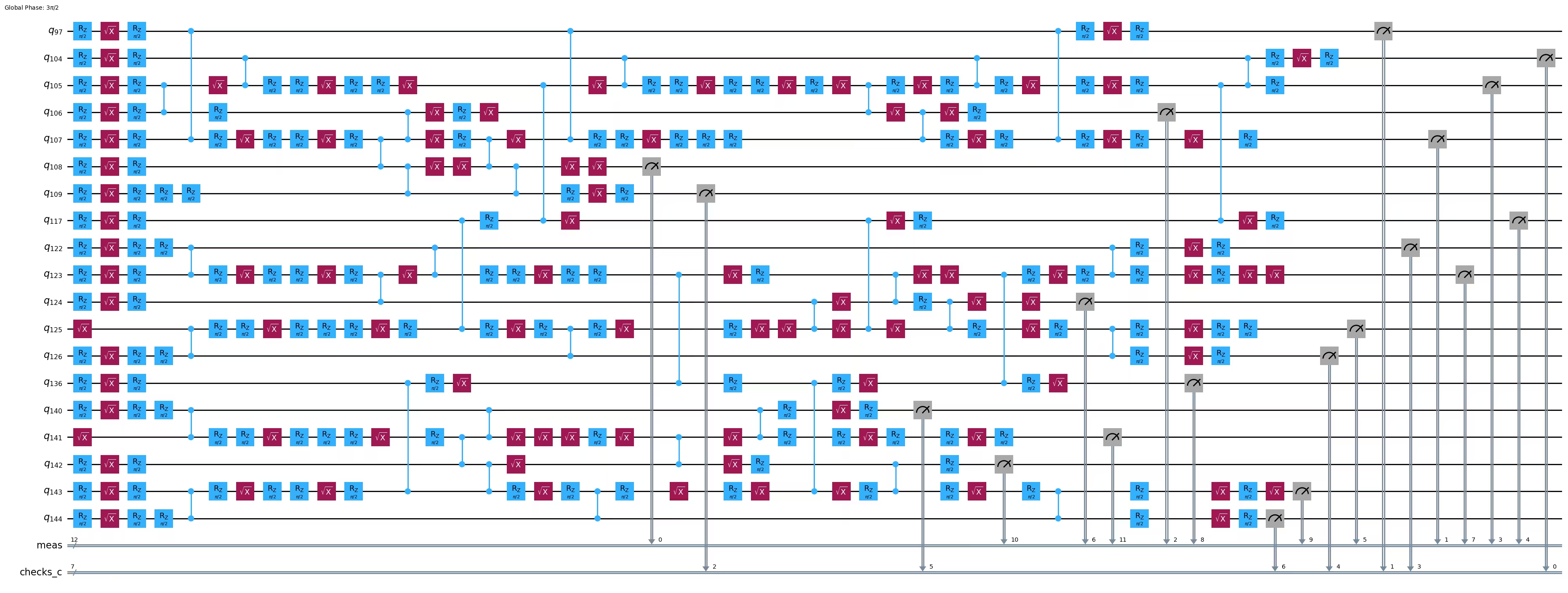
Output dari add_pauli_checks adalah urutan circuit dengan jumlah check yang meningkat, dari tanpa check hingga satu check pada setiap qubit target. Visualisasi mengonfirmasi bahwa check menggunakan pasangan target dan ancilla yang ditentukan. Untuk detail tentang menemukan check yang baik, lihat Bagian II hingga IV dari informasi tambahan dalam referensi [1].

checked = add_pauli_checks(
    circuit_isa,
    target_qubits,
    noise_model,
    ancilla_qubits=ancilla_qubits,
    cost="gamma",
    method="windowed",
    seed=seed,
)

print(f"Physical layout of payload and ancillas: {layout + ancilla_qubits}")
print("Checked circuit:")
checked[-1].circuit.draw("mpl", fold=-1, idle_wires=False)

Physical layout of payload and ancillas: [108, 107, 106, 105, 117, 125, 124, 123, 136, 143, 142, 141, 104, 97, 109, 122, 126, 140, 144]
Checked circuit:

Langkah 3: Mengeksekusi menggunakan primitive Qiskit

Untuk membuat efek noise gate terlihat, tingkatkan kedalaman payload dan sampel sebagian dari stabilizer-nya. Setiap stabilizer umumnya tidak qubit-wise commuting dengan yang lain, sehingga satu set check tidak valid untuk dua stabilizer yang berbeda. Alih-alih mengelompokkan stabilizer ke dalam set yang commuting, temukan set check yang baik untuk setiap stabilizer secara independen. Menyampel stabilizer secara seragam acak memberikan estimasi fidelitas yang tidak bias.

Bangun circuit yang lebih dalam dan ambil sampel acak dari stabilizer-nya.

depth = 24
num_stabilizers = 20
num_shots = 1_000

circuit = random_clifford_circuit(num_qubits, depth, rng)

# Build the full stabilizer group, then sample from it uniformly at random
circ_no_meas = circuit.remove_final_measurements(inplace=False)
stabilizer_group = PauliList([Pauli("I" * num_qubits)])
for generator in (
    Pauli(label) for label in Clifford(circ_no_meas).to_labels(mode="S")
):
    stabilizer_group = stabilizer_group + stabilizer_group.compose(generator)

keep = np.where(
    stabilizer_group.x.any(axis=1) | stabilizer_group.z.any(axis=1)
)[0]
chosen = np.random.default_rng(seed).choice(
    keep, size=min(num_stabilizers, len(keep)), replace=False
)
stabilizers = [stabilizer_group[int(i)] for i in chosen]

two_qubit_depth = circuit.depth(lambda x: x.operation.num_qubits == 2)
print(
    f"Sampled {len(stabilizers)} stabilizers of a {circuit.num_qubits}-qubit "
    f"circuit with two-qubit depth {two_qubit_depth}: "
    f"{{{stabilizers[0]}, {stabilizers[1]}, ...}}"
)

Sampled 20 stabilizers of a 12-qubit circuit with two-qubit depth 24: {ZXIIXZYYXIZZ, XXXYIIZYXIII, ...}

Untuk setiap stabilizer yang disampel, rotasikan circuit sehingga stabilizer diukur dalam basis komputasi, transpile ke backend, dan temukan set check yang baik. Pasangan target dan ancilla diacak bersama untuk setiap stabilizer sehingga setiap target mempertahankan ancilla-nya. Ingat bahwa check dikomit secara berurutan dalam urutan qubit target diberikan, dan check yang telah dikomit tidak berubah seiring lebih banyak check ditambahkan.

noisy_circuits = []
checked_circuits = []
depths_2q = []
t0 = time.time()
for i, pauli in enumerate(tqdm(stabilizers)):
    noisy_circuits.append(pm.run(append_basis_rotation(circuit, pauli)))
    # Shuffle target and ancilla pairs together so each target keeps its ancilla
    targets, ancillas = zip(
        *random.sample(
            list(zip(target_qubits, ancilla_qubits, strict=True)),
            k=len(target_qubits),
        ),
        strict=True,
    )
    checked_circuits.append(
        add_pauli_checks(
            noisy_circuits[-1],
            list(targets),
            noise_model,
            ancilla_qubits=list(ancillas),
            cost="gamma",
            method="windowed",
            seed=seed + 1 + i,
        )
    )
    depths_2q.append(
        checked_circuits[-1][-1].circuit.depth(lambda x: len(x.qubits) == 2)
    )

print(
    f"Added {num_checks} checks to {len(stabilizers)} circuits "
    f"in {(time.time() - t0):.0f}s."
)
print(
    f"On average, two-qubit depth increased from "
    f"{circuit.depth(lambda x: len(x.qubits) == 2)} to {int(np.mean(depths_2q))} "
    f"when adding {num_checks} checks."
)

100%|██████████| 20/20 [00:15<00:00,  1.29it/s]

Added 7 checks to 20 circuits in 15s.
On average, two-qubit depth increased from 24 to 33 when adding 7 checks.

Sampel payload polos dan circuit yang telah dicheck dengan Qiskit Aer. Simulator menggunakan model depolarizing yang sama yang menilai check, sehingga noise yang ditargetkan oleh check adalah noise yang diterapkan simulator.

aer_nm = AerNoiseModel()
aer_nm.add_all_qubit_quantum_error(
    depolarizing_error(noise_model.gate_noise, 2), ["cz"]
)
p = noise_model.readout_noise
aer_nm.add_all_qubit_readout_error(ReadoutError([[1 - p, p], [p, 1 - p]]))
noisy_sim = AerSimulator(method="stabilizer", noise_model=aer_nm)

counts = []
for i, checked_circ_result in enumerate(tqdm(checked_circuits)):
    noisy_counts = (
        noisy_sim.run(
            noisy_circuits[i], shots=num_shots, seed_simulator=seed * i + 1
        )
        .result()
        .get_counts()
    )
    checked_counts_per_variant = []
    for k, ck in enumerate(checked_circ_result):
        variant_counts = (
            noisy_sim.run(
                ck.circuit, shots=num_shots, seed_simulator=seed * i + 2 + k
            )
            .result()
            .get_counts()
        )
        checked_counts_per_variant.append(variant_counts)
    counts.append((noisy_counts, checked_counts_per_variant))

100%|██████████| 20/20 [00:17<00:00,  1.13it/s]

Langkah 4: Pasca-pemrosesan dan mengembalikan hasil dalam format klasik yang diinginkan

Setiap check menggunakan entangling gate antara satu ancilla dan satu target. Ancilla dimulai pada $|0\rangle$, sehingga $Z_\text{anc}$ menstabilkan inputnya. Menjalankan $Z_\text{anc}$ maju melalui circuit yang telah dicheck menghasilkan operator Pauli pada output yang suku non-identitasnya mendefinisikan support check tersebut. Sebuah check lolos ketika bit dalam support-nya memiliki paritas genap. Sampel disimpan hanya ketika setiap check lolos.

get_postselection_method dari setiap CheckedCircuit mengembalikan fungsi yang memetakan bitstring yang diukur ke vektor syndrome. Simpan sampel yang syndrome-nya nol untuk setiap check, dan buang sisanya. Grafik yang mengikuti menunjukkan bahwa menambah lebih banyak check menurunkan laju postselection. Laju postselection yang lebih rendah membutuhkan lebih banyak shot untuk mencapai akurasi target, sehingga ada tradeoff antara kemampuan deteksi dan biaya sampling. Laju tampak konvergen, yang menunjukkan bahwa check tambahan berkontribusi lebih sedikit kemampuan deteksi.

rate_per_variant = []
kept_per_stab = []
for i, (_, checked_counts_per_variant) in enumerate(counts):
    rates = []
    kept_at_num_checks = None
    for k, variant_counts in enumerate(checked_counts_per_variant):
        ps_fn = checked_circuits[i][k].get_postselection_method()
        kept = {
            bs: n for bs, n in variant_counts.items() if not ps_fn(bs).any()
        }
        rates.append(sum(kept.values()) / num_shots)
        if k == num_checks:
            kept_at_num_checks = kept
    rate_per_variant.append(rates)
    kept_per_stab.append(kept_at_num_checks)

max_len = max(len(s) for s in rate_per_variant)
rates_arr = np.full((len(rate_per_variant), max_len), np.nan)
for i, s in enumerate(rate_per_variant):
    rates_arr[i, : len(s)] = s
ks = np.arange(max_len)

fig, ax = plt.subplots(figsize=(8, 4))
ax.plot(ks, rates_arr.T, color="#ff8c00", alpha=0.15, linewidth=1)
ax.plot(
    ks,
    np.nanmedian(rates_arr, axis=0),
    color="black",
    linewidth=1,
    linestyle="--",
    label="median",
)
ax.set_xlabel("Checks committed")
ax.set_ylabel("Postselection rate")
ax.set_ylim((0, 1.05))
ax.set_title(
    f"Per-stabilizer postselection rate ({len(rates_arr)} stabilizers)"
)
ax.legend()
ax.grid(True, alpha=0.3)
plt.tight_layout()
plt.show()

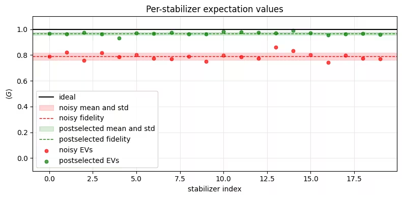
Sekarang bandingkan fidelitas state noisy polos dengan state yang telah di-postselect. Melakukan postselect hanya pada sampel tanpa error yang terdeteksi meningkatkan nilai ekspektasi setiap stabilizer, dan karenanya estimasi fidelitas. Nilai yang telah di-postselect menggunakan lebih sedikit sampel dibandingkan nilai mentah, namun nilai ekspektasinya lebih akurat dan variansi yang disampel lebih rendah. Perhatikan juga bahwa laju postselection rata-rata mendekati fidelitas noisy. Ini yang diharapkan ketika check mendeteksi hampir semua sampel yang salah: fraksi sampel yang lolos setiap check mendekati fraksi sampel bebas-error, yang merupakan fidelitas dari state noisy.

results = []
for i, ((noisy_counts, _), kept) in enumerate(
    zip(counts, kept_per_stab, strict=True)
):
    results.append(
        (
            expectation(noisy_counts, stabilizers[i]),
            expectation(kept, stabilizers[i]),
            sum(kept.values()) / num_shots,
        )
    )

fidelity_noisy = float(np.nanmean([r[0] for r in results]))
fidelity_postsel = float(np.nanmean([r[1] for r in results]))
psr = float(np.mean([r[2] for r in results]))
print(
    f"ideal fidelity:          1.0\n"
    f"noisy fidelity:          {fidelity_noisy:.4f}\n"
    f"postselected fidelity:   {fidelity_postsel:.4f}\n"
    f"mean postselection rate: {psr:.3f}"
)

evs_ideal = np.ones(len(results))
evs_noisy = np.array([r[0] for r in results])
evs_post = np.array([r[1] for r in results])
idx = np.arange(len(results))

def strip(ax, ys, color, label):
    m, s = np.nanmean(ys), np.nanstd(ys)
    ax.axhspan(
        m - s, m + s, color=color, alpha=0.15, label=f"{label} mean and std"
    )
    ax.axhline(
        m, color=color, linewidth=1, linestyle="--", label=f"{label} fidelity"
    )

fig, ax = plt.subplots(figsize=(8, 4))
ax.axhline(np.nanmean(evs_ideal), color="black", linewidth=1.5, label="ideal")
strip(ax, evs_noisy, "red", "noisy")
strip(ax, evs_post, "green", "postselected")
ax.scatter(idx, evs_noisy, color="red", s=22, alpha=0.7, label="noisy EVs")
ax.scatter(
    idx,
    evs_post,
    color="green",
    s=22,
    alpha=0.7,
    label="postselected EVs",
)
ax.set_xlabel("stabilizer index")
ax.set_ylabel(r"$\langle G \rangle$")
ax.set_ylim((-0.1, 1.1))
ax.set_title("Per-stabilizer expectation values")
ax.legend(loc="lower left")
ax.grid(True, alpha=0.3)
plt.tight_layout()
plt.show()

M = np.arange(1, len(results) + 1)
fig, ax = plt.subplots(figsize=(8, 4))
for ys, color, label in [
    (evs_ideal, "black", "ideal"),
    (evs_noisy, "red", "noisy"),
    (evs_post, "green", "postselected"),
]:
    cm, sem = cum_mean_sem(ys)
    ax.plot(M, cm, color=color, linewidth=1.5, label=label)
    ax.fill_between(M, cm - sem, cm + sem, color=color, alpha=0.15)
ax.set_xlabel("number of stabilizers averaged")
ax.set_ylabel("running fidelity estimate")
ax.set_title("Fidelity convergence versus number of stabilizers")
ax.legend()
ax.grid(True, alpha=0.3)
plt.tight_layout()
plt.show()

ideal fidelity:          1.0
noisy fidelity:          0.7899
postselected fidelity:   0.9679
mean postselection rate: 0.780

Skor gamma melaporkan seberapa banyak kanal noise yang dimodelkan tetap tidak terdeteksi oleh check. Memplot skor gamma terhadap jumlah check yang dikomit menunjukkan bagaimana kemampuan deteksi meningkat seiring setiap check ditambahkan. Nilai 1.0 berarti check menangkap semua noise yang dimodelkan. Kurva turun menuju 1.0 seiring lebih banyak check dikomit, yang menunjukkan bahwa setiap check tambahan menangkap sebagian error yang belum terdeteksi.

stab_scores = [
    [variant.cost for variant in checked_circ_result]
    for checked_circ_result in checked_circuits
]
max_len = max(len(s) for s in stab_scores)
scores = np.full((len(stab_scores), max_len), np.nan)
for i, s in enumerate(stab_scores):
    scores[i, : len(s)] = s
ks = np.arange(max_len)

fig, ax = plt.subplots(figsize=(8, 4))
ax.plot(ks, scores.T, color="#4682b4", alpha=0.15, linewidth=1)
ax.plot(
    ks,
    np.nanmedian(scores, axis=0),
    color="black",
    linewidth=1,
    linestyle="--",
    label="median",
)
ax.set_xlabel("Checks committed")
ax.set_ylabel("Gamma")
ax.set_yscale("log")
ax.set_title(f"Per-stabilizer gamma curves ({len(scores)} stabilizers)")
ax.legend()
ax.grid(True, alpha=0.3, which="both")
plt.tight_layout()
plt.show()

Contoh hardware skala besar

Alur kerja yang sama berjalan pada hardware dengan payload yang lebih besar dan lebih dalam. Bagian ini menggunakan kembali backend dari contoh simulator tetapi membangun layout 20-qubit baru dengan pasangan target dan ancilla serta pass manager-nya sendiri, kemudian mengirimkan circuit ke QPU dalam satu job tunggal. Pada ukuran ini, sebagian besar shot memicu setidaknya satu check, sehingga laju postselection rendah, dan setiap circuit membutuhkan budget shot yang besar untuk cukup sampel yang bertahan. Contoh ini karenanya memfokuskan budget-nya pada beberapa stabilizer yang disampel; ini masih merupakan estimasi fidelitas yang tidak bias, tetapi lebih kasar dibandingkan rata-rata contoh simulator atas banyak stabilizer.

Satu hal berubah relatif terhadap contoh simulator: alih-alih menyimpulkan kanal depolarizing seragam dari data kalibrasi, bagian ini mempelajari model noise dengan NoiseLearner dan membangun model qiskit-paulice dari hasilnya dengan NoiseModel.from_pauli_lindblad_maps. Model Pauli-Lindblad yang dipelajari menangkap struktur spasial noise pada layout spesifik ini, alih-alih mengasumsikan setiap edge sama noisy-nya, sehingga penempatan check dinilai terhadap noise yang lebih mirip dengan yang memengaruhi QPU. Mempelajari noise membutuhkan sampling QPU dan harus diperhitungkan dalam budget sampling QPU secara keseluruhan.

Parameter yang mengikuti mengatur jumlah qubit, kedalaman, jumlah stabilizer, dan jumlah shot. Skalakan hw_num_shots dengan kebalikan dari laju postselection: pada laju 3%, 40.000 shot menyisakan sekitar 1.200 sampel yang telah di-postselect per circuit. Tingkatkan hw_num_stabilizers untuk estimasi fidelitas yang lebih presisi dengan biaya lebih banyak circuit per job, yang masing-masing membutuhkan budget shot yang sama.

Langkah 1-4 (dikompresi menjadi satu blok kode)

Sel berikut menjalankan empat langkah yang sama seperti contoh simulator. Ini membangun payload yang lebih besar dan menyampel beberapa stabilizer (langkah 1); memilih layout, mempelajari model noise-nya, dan menemukan circuit yang telah sepenuhnya dicheck untuk setiap stabilizer (langkah 2); mengirimkan satu job Sampler yang berisi circuit polos dan yang telah dicheck (langkah 3); dan melakukan postselect pada counts yang telah dicheck untuk membandingkan estimasi fidelitas noisy dan postselected, per stabilizer dan rata-rata (langkah 4). Pada ukuran ini, mengenumerasi seluruh grup stabilizer seperti contoh simulator tidak layak, sehingga sel ini melakukan subsampling subset acak stabilizer untuk menghitung estimasi fidelitas.

Perhatikan bahwa langkah 2 melakukan lebih banyak di sini dibandingkan pada contoh simulator: mempelajari model noise mengirimkan job NoiseLearner-nya sendiri sebelum job Sampler, sehingga sel ini menjalankan dua job secara total. Mereka membawa tag TUT_ASPC_LEARN dan TUT_ASPC sehingga Anda dapat menemukannya nanti. Lihat Mengorganisasi dan mencari berdasarkan tag job untuk info lebih lanjut tentang pemberian tag pada job.

# -------------------------Step 1: build a larger payload and sample stabilizers-------------------------
hw_num_qubits = 20
hw_depth = 36
hw_num_stabilizers = 10
hw_num_shots = 40_000

hw_circuit = random_clifford_circuit(hw_num_qubits, hw_depth, rng)
hw_no_meas = hw_circuit.remove_final_measurements(inplace=False)

# Enumerating all 2^n stabilizers is infeasible at this size, so draw each
# stabilizer by composing a random subset of the group generators
hw_generators = [
    Pauli(label) for label in Clifford(hw_no_meas).to_labels(mode="S")
]
sample_rng = np.random.default_rng(seed)
hw_stabilizers = []
while len(hw_stabilizers) < hw_num_stabilizers:
    mask = sample_rng.integers(0, 2, hw_num_qubits).astype(bool)
    if not mask.any():
        continue  # skip the identity
    stabilizer = Pauli("I" * hw_num_qubits)
    for generator, chosen in zip(hw_generators, mask, strict=True):
        if chosen:
            stabilizer = stabilizer.compose(generator)
    hw_stabilizers.append(stabilizer)

# -------------------------Step 2: find a 20-qubit layout, learn its noise, and add checks-------------------------
# A single bad coupler or bad-readout qubit on the path drags every
# stabilizer down, so search harder and with tighter error thresholds
hw_layout = find_check_layout(
    backend,
    hw_num_qubits,
    rng,
    num_trials=500,
    max_gate_error=0.015,
    max_readout_error=0.05,
)
hw_target_qubits, hw_ancilla_qubits = get_check_qubits(backend, hw_layout)
hw_pm = generate_preset_pass_manager(
    optimization_level=0, backend=backend, initial_layout=hw_layout
)
print(f"Layout with {len(hw_target_qubits)} check pairs: {hw_layout}")

# ----- learn a Pauli-Lindblad noise model on this layout -----
# The simulator example scored checks against a uniform depolarizing channel
# inferred from calibration data. Here, learn the noise instead: NoiseLearner
# runs its own job on the QPU and returns a Pauli-Lindblad channel per unique
# entangling layer, so the checks are placed against the noise this layout
# actually has, including its spatial structure. All the sampled stabilizers
# share the same entangling layers and differ only in their final basis
# rotation, so learning on the bare payload covers all of them.
learner = NoiseLearner(
    mode=backend,
    options={
        "max_layers_to_learn": 4,
        "num_randomizations": 32,
        "shots_per_randomization": 128,
        "environment": {"job_tags": ["TUT_ASPC_LEARN"]},
    },
)
learner_job = learner.run([hw_pm.run(hw_circuit)])
print(f"Submitted noise-learner job {learner_job.job_id()}")
hw_layer_errors = learner_job.result().data

# To see how much the learned model helps, swap the next line for the
# simulator example's uniform model - a one-line change:
# hw_noise_model = NoiseModel.from_backend(backend, hw_layout, uniform_gate_noise=True)
hw_noise_model = learned_noise_model(hw_layer_errors, hw_layout)
# NoiseLearner characterizes gate noise only, so keep the readout estimate
# from calibration data rather than leaving it unset
hw_noise_model.readout_noise = NoiseModel.from_backend(
    backend, hw_layout, uniform_gate_noise=True
).readout_noise
print(
    f"Learned {len(hw_layer_errors)} layers; "
    f"readout noise {hw_noise_model.readout_noise:.5f}"
)

# ----- add the fully checked circuit per stabilizer -----
hw_noisy_circuits = []
hw_checked_circuits = []
for i, pauli in enumerate(tqdm(hw_stabilizers)):
    bare = hw_pm.run(append_basis_rotation(hw_circuit, pauli))
    hw_noisy_circuits.append(bare)
    variants = add_pauli_checks(
        bare,
        hw_target_qubits,
        hw_noise_model,
        ancilla_qubits=hw_ancilla_qubits,
        cost="gamma",
        method="windowed",
        seed=seed + 1 + i,
    )
    hw_checked_circuits.append(variants[-1])  # keep the fully checked circuit

# -------------------------Step 3: submit one Sampler job with the bare and checked circuits-------------------------
sampler = Sampler(mode=backend)
sampler.options.default_shots = hw_num_shots
sampler.options.environment.job_tags = ["TUT_ASPC"]

pubs = hw_noisy_circuits + [cc.circuit for cc in hw_checked_circuits]
job = sampler.run(pubs)
print(f"Submitted job {job.job_id()} with {len(pubs)} circuits")

# -------------------------Step 4: postselect and compare fidelity-------------------------
result = job.result()
n_stab = len(hw_stabilizers)

hw_results = []
for i in range(n_stab):
    noisy_counts = result[i].join_data().get_counts()
    checked_counts = result[n_stab + i].join_data().get_counts()
    ps_fn = hw_checked_circuits[i].get_postselection_method()
    kept = {bs: c for bs, c in checked_counts.items() if not ps_fn(bs).any()}
    hw_results.append(
        (
            expectation(noisy_counts, hw_stabilizers[i]),
            expectation(kept, hw_stabilizers[i]),
            sum(kept.values()) / sum(checked_counts.values()),
        )
    )

hw_fidelity_noisy = float(np.nanmean([r[0] for r in hw_results]))
hw_fidelity_postsel = float(np.nanmean([r[1] for r in hw_results]))
hw_psr = float(np.mean([r[2] for r in hw_results]))
print(
    f"noisy fidelity estimate:        {hw_fidelity_noisy:.4f}\n"
    f"postselected fidelity estimate: {hw_fidelity_postsel:.4f}\n"
    f"mean postselection rate:        {hw_psr:.4f} "
    f"(~{int(round(hw_psr * hw_num_shots))} kept shots per circuit)"
)

# Per-stabilizer breakdown. The postselection rate varies from stabilizer to
# stabilizer, so a stabilizer whose postselected value barely moves is usually
# one whose checks rejected little; the kept-shot count says how much of the
# gap is statistics rather than signal.
print("\nper-stabilizer results:")
print(
    f"{'idx':>3}  {'noisy':>8}  {'postsel':>8}  {'psr':>7}  {'kept shots':>10}"
)
for i, (noisy, post, psr_i) in enumerate(hw_results):
    print(
        f"{i:>3}  {noisy:>8.4f}  {post:>8.4f}  {psr_i:>7.4f}  "
        f"{int(round(psr_i * hw_num_shots)):>10}"
    )

hw_noisy = np.array([r[0] for r in hw_results])
hw_post = np.array([r[1] for r in hw_results])
idx = np.arange(n_stab)

fig, ax = plt.subplots(figsize=(9, 4))
ax.axhline(1.0, color="black", linewidth=1.5, label="ideal")
strip(ax, hw_noisy, "red", "noisy")
strip(ax, hw_post, "green", "postselected")
ax.scatter(idx, hw_noisy, color="red", s=22, alpha=0.7, label="noisy EVs")
ax.scatter(
    idx,
    hw_post,
    color="green",
    s=22,
    alpha=0.7,
    label="postselected EVs",
)
ax.set_xlabel("stabilizer index")
ax.set_ylabel(r"$\langle G \rangle$")
ax.set_ylim((-0.1, 1.1))
ax.set_xticks(idx)
ax.set_title("Per-stabilizer expectation values on hardware")
# Outside the axes so it cannot hide a data point
ax.legend(loc="center left", bbox_to_anchor=(1.02, 0.5), frameon=False)
ax.grid(True, alpha=0.3)
plt.tight_layout()
plt.show()

Layout with 11 check pairs: [153, 152, 151, 138, 131, 130, 129, 118, 109, 110, 111, 98, 91, 90, 89, 78, 69, 70, 71, 58]
Submitted noise-learner job d9f4mncjeosc73fjfmkg

Learned 4 layers; readout noise 0.00470

100%|██████████| 10/10 [01:01<00:00,  6.18s/it]

Submitted job d9f4s04jeosc73fjftkg with 20 circuits
noisy fidelity estimate:        0.3685
postselected fidelity estimate: 0.6869
mean postselection rate:        0.2851 (~11404 kept shots per circuit)

per-stabilizer results:
idx     noisy   postsel      psr  kept shots
  0    0.3769    0.6918   0.3247       12987
  1    0.3745    0.6760   0.2999       11995
  2    0.3659    0.6389   0.3549       14196
  3    0.3821    0.7060   0.2660       10641
  4    0.3653    0.7475   0.2531       10124
  5    0.3752    0.7022   0.2698       10791
  6    0.3508    0.7144   0.2711       10842
  7    0.3485    0.7087   0.2381        9523
  8    0.3825    0.6289   0.2928       11711
  9    0.3630    0.6549   0.2808       11232

Untuk circuit dengan ukuran ini, sebagian besar sampel mengandung setidaknya satu error yang terdeteksi, sehingga laju postselection kecil dan postselection membuang sebagian besar shot. Sampel yang lolos setiap check memberikan nilai ekspektasi yang jauh lebih baik dibandingkan circuit polos, dan nilai per-stabilizer terpisah dengan jelas dari baseline noisy. Untuk memperketat estimasi fidelitas, sampel lebih banyak stabilizer dengan budget shot per-circuit yang sama. Untuk meningkatkan laju postselection, kurangi kedalaman circuit atau komit lebih sedikit check; untuk mendorong ke payload yang lebih besar, skalakan budget shot dengan kebalikan laju postselection.

Langkah selanjutnya

Rekomendasi

Jika Anda merasa pekerjaan ini menarik, Anda mungkin tertarik dengan materi berikut:

• Tutorial tentang repetition codes untuk pengenalan koreksi error kuantum.

• Dokumentasi qiskit-paulice untuk API pencarian check yang lengkap, dan repositori GitHub paket ini untuk kode sumbernya.

• Makalah Low-overhead error detection with spacetime codes untuk teori di balik check.

Referensi

• [1] Martiel, S., & Javadi-Abhari, A. (2025). Low-overhead error detection with spacetime codes. arXiv preprint arXiv:2504.15725.

• [2] van den Berg, E., Bravyi, S., Gambetta, J. M., Jurcevic, P., Maslov, D., & Temme, K. (2023). Single-shot error mitigation by coherent Pauli checks. Physical Review Research, 5(3), 033193.