Formula multi-produk untuk mengurangi kesalahan Trotter

Perkiraan penggunaan QPU: Empat menit pada prosesor Heron r2 (CATATAN: Ini hanya perkiraan. Waktu aktual kamu bisa berbeda.)

Latar Belakang

Tutorial ini menunjukkan cara menggunakan Formula Multi-Produk (MPF) untuk mencapai kesalahan Trotter yang lebih rendah pada observabel dibandingkan dengan yang ditimbulkan oleh Circuit Trotter terdalam yang akan kita jalankan. MPF mengurangi kesalahan Trotter dari dinamika Hamiltonian melalui kombinasi berbobot dari beberapa eksekusi Circuit. Pertimbangkan tugas mencari nilai ekspektasi observabel untuk keadaan kuantum $\rho(t)=e^{-i H t} \rho(0) e^{i H t}$ dengan Hamiltonian $H$. Kita bisa menggunakan Formula Produk (PF) untuk mengaproksimasi evolusi waktu $e^{-i H t}$ dengan cara berikut:

• Tulis Hamiltonian $H$ sebagai $H=\sum_{a=1}^d F_a,$ di mana $F_a$ adalah operator Hermitian sehingga setiap uniter yang bersesuaian bisa diimplementasikan secara efisien pada perangkat kuantum.
• Aproksimasi suku $F_a$ yang tidak komutasi satu sama lain.

Kemudian, PF orde pertama (formula Lie-Trotter) adalah:

$S_1(t):=\prod_{a=1}^d e^{-i F_a t},$

yang memiliki suku kesalahan kuadratik $S_1(t)=e^{-i H t}+\mathcal{O}\left(t^{2}\right)$. Kita juga bisa menggunakan PF orde lebih tinggi (formula Lie-Trotter-Suzuki), yang konvergen lebih cepat, dan didefinisikan secara rekursif sebagai:

$S_2(t):=\prod_{a=1}^d e^{-i F_a t/2}\prod_{a=1}^d e^{-i F_a t/2}$

$S_{2 \chi}(t):= S_{2 \chi -2}(s_{\chi}t)^2 S_{2 \chi -2}((1-4s_{\chi})t)S_{2 \chi -2}(s_{\chi}t)^2,$

di mana $\chi$ adalah orde PF simetrik dan $s_p = \left( 4 - 4^{1/(2p-1)} \right)^{-1}$. Untuk evolusi waktu panjang, kita bisa membagi interval waktu $t$ menjadi $k$ interval, yang disebut langkah Trotter, berdurasi $t/k$ dan mengaproksimasi evolusi waktu di setiap interval dengan formula produk orde $\chi$, yaitu $S_{\chi}$. Dengan demikian, PF orde $\chi$ untuk operator evolusi waktu selama $k$ langkah Trotter adalah:

$S_{\chi}^{k}(t) = \left[ S_{\chi} \left( \frac{t}{k} \right)\right]^k = e^{-i H t}+O\left(t \left( \frac{t}{k} \right)^{\chi} \right)$

di mana suku kesalahan berkurang seiring bertambahnya jumlah langkah Trotter $k$ dan orde $\chi$ dari PF.

Diberikan bilangan bulat $k \geq 1$ dan formula produk $S_{\chi}(t)$, keadaan terevolvsi-waktu aproksimasi $\rho_k(t)$ bisa diperoleh dari $\rho_0$ dengan menerapkan $k$ iterasi dari formula produk $S_{\chi}\left(\frac{t}{k}\right)$.

$$\rho_k(t)=S_{\chi}\left(\frac{t}{k}\right)^k \rho_0 S_{\chi}\left(\frac{t}{k}\right)^{-k}$$

$\rho_k(t)$ adalah aproksimasi dari $\rho(t)$ dengan kesalahan aproksimasi Trotter ||$\rho_k(t)-\rho(t) ||$. Jika kita mempertimbangkan kombinasi linear dari aproksimasi Trotter $\rho(t)$:

$$\mu(t) = \sum_{j}^{l} x_j \rho^{k_j}_{j}\left(\frac{t}{k_j}\right) + \text{some remaining Trotter error} \, ,$$

di mana $x_j$ adalah koefisien pembobot kita, $\rho^{k_j}_j$ adalah matriks densitas yang sesuai dengan keadaan murni yang diperoleh dengan mengevolusikan keadaan awal menggunakan formula produk, $S^{k_j}_{\chi}$, yang melibatkan $k_j$ langkah Trotter, dan $j \in {1, ..., l}$ mengindeks jumlah PF yang membentuk MPF. Semua suku dalam $\mu(t)$ menggunakan formula produk $S_{\chi}(t)$ yang sama sebagai dasarnya. Tujuannya adalah untuk memperbaiki ||$\rho_k(t)-\rho(t) \|$ dengan menemukan $\mu(t)$ yang memiliki $\|\mu(t)-\rho(t)\|$ lebih rendah.

• $\mu(t)$ tidak harus berupa keadaan fisik karena $x_i$ tidak harus positif. Tujuan di sini adalah meminimalkan kesalahan dalam nilai ekspektasi observabel, bukan mencari pengganti fisik untuk $\rho(t)$.
• $k_j$ menentukan kedalaman Circuit dan tingkat aproksimasi Trotter. Nilai $k_j$ yang lebih kecil menghasilkan Circuit yang lebih pendek, yang menimbulkan lebih sedikit kesalahan Circuit tetapi akan menjadi aproksimasi yang kurang akurat terhadap keadaan yang diinginkan.

Kunci di sini adalah bahwa sisa kesalahan Trotter yang diberikan oleh $\mu(t)$ lebih kecil dari kesalahan Trotter yang akan diperoleh dengan hanya menggunakan nilai $k_j$ terbesar.

Kamu bisa melihat kegunaan ini dari dua perspektif:

1. Untuk anggaran langkah Trotter yang tetap yang bisa kamu jalankan, kamu bisa memperoleh hasil dengan kesalahan Trotter yang lebih kecil secara total.
2. Diberikan suatu target jumlah langkah Trotter yang terlalu besar untuk dijalankan, kamu bisa menggunakan MPF untuk menemukan kumpulan Circuit berkedalaman lebih rendah yang dijalankan dan menghasilkan kesalahan Trotter serupa.

Persyaratan

Sebelum memulai tutorial ini, pastikan kamu sudah menginstal hal-hal berikut:

• Qiskit SDK v1.0 atau lebih baru, dengan dukungan visualisasi
• Qiskit Runtime v0.22 atau lebih baru (pip install qiskit-ibm-runtime)
• MPF Qiskit addons (pip install qiskit_addon_mpf)
• Qiskit addons utils (pip install qiskit_addon_utils)
• Library Quimb (pip install quimb)
• Library Qiskit Quimb (pip install qiskit-quimb)
• Numpy v0.21 untuk kompatibilitas antar paket (pip install numpy==0.21)

Bagian I. Contoh skala kecil

Jelajahi stabilitas MPF

Tidak ada batasan jelas pada pilihan jumlah langkah Trotter $k_j$ yang membentuk keadaan MPF $\mu(t)$. Namun, ini harus dipilih dengan hati-hati untuk menghindari ketidakstabilan dalam nilai ekspektasi yang dihitung dari $\mu(t)$. Aturan umum yang baik adalah menetapkan langkah Trotter terkecil $k_{\text{min}}$ sehingga $t/k_{\text{min}} \lt 1$. Kalau kamu ingin belajar lebih lanjut tentang ini dan cara memilih nilai $k_j$ lainnya, lihat panduan Cara memilih langkah Trotter untuk MPF.

Dalam contoh di bawah ini, kita menjelajahi stabilitas solusi MPF dengan menghitung nilai ekspektasi magnetisasi untuk berbagai waktu menggunakan keadaan terevolvsi-waktu yang berbeda. Secara khusus, kita membandingkan nilai ekspektasi yang dihitung dari setiap aproksimasi evolusi waktu yang diimplementasikan dengan langkah Trotter yang bersesuaian dan berbagai model MPF (koefisien statis dan dinamis) dengan nilai eksak dari observabel terevolvsi-waktu. Pertama, mari kita definisikan parameter untuk formula Trotter dan waktu evolusi

# Added by doQumentation — required packages for this notebook
!pip install -q matplotlib numpy qiskit qiskit-addon-mpf qiskit-addon-utils qiskit-aer qiskit-ibm-runtime rustworkx scipy

import numpy as np

mpf_trotter_steps = [1, 2, 4]
order = 2
symmetric = False

trotter_times = np.arange(0.5, 1.55, 0.1)
exact_evolution_times = np.arange(trotter_times[0], 1.55, 0.05)

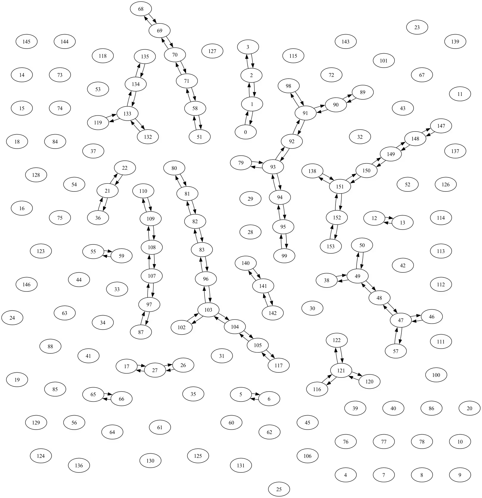
Untuk contoh ini, kita akan menggunakan keadaan Neel sebagai keadaan awal $\vert \text{Neel} \rangle = \vert 0101...01 \rangle$ dan model Heisenberg pada garis 10 titik untuk Hamiltonian yang mengatur evolusi waktu

$$\hat{\mathcal{H}}_{Heis} = J \sum_{i=1}^{L-1} \left(X_i X_{(i+1)}+Y_i Y_{(i+1)}+ Z_i Z_{(i+1)} \right) \, ,$$

di mana $J$ adalah kekuatan kopling untuk tepi tetangga terdekat.

from qiskit.transpiler import CouplingMap
from rustworkx.visualization import graphviz_draw
from qiskit_addon_utils.problem_generators import generate_xyz_hamiltonian
import numpy as np

L = 10

# Generate some coupling map to use for this example
coupling_map = CouplingMap.from_line(L, bidirectional=False)
graphviz_draw(coupling_map.graph, method="circo")

# Get a qubit operator describing the Heisenberg field model
hamiltonian = generate_xyz_hamiltonian(
    coupling_map,
    coupling_constants=(1.0, 1.0, 1.0),
    ext_magnetic_field=(0.0, 0.0, 0.0),
)

print(hamiltonian)

SparsePauliOp(['IIIIIIIXXI', 'IIIIIIIYYI', 'IIIIIIIZZI', 'IIIIIXXIII', 'IIIIIYYIII', 'IIIIIZZIII', 'IIIXXIIIII', 'IIIYYIIIII', 'IIIZZIIIII', 'IXXIIIIIII', 'IYYIIIIIII', 'IZZIIIIIII', 'IIIIIIIIXX', 'IIIIIIIIYY', 'IIIIIIIIZZ', 'IIIIIIXXII', 'IIIIIIYYII', 'IIIIIIZZII', 'IIIIXXIIII', 'IIIIYYIIII', 'IIIIZZIIII', 'IIXXIIIIII', 'IIYYIIIIII', 'IIZZIIIIII', 'XXIIIIIIII', 'YYIIIIIIII', 'ZZIIIIIIII'],
              coeffs=[1.+0.j, 1.+0.j, 1.+0.j, 1.+0.j, 1.+0.j, 1.+0.j, 1.+0.j, 1.+0.j, 1.+0.j,
 1.+0.j, 1.+0.j, 1.+0.j, 1.+0.j, 1.+0.j, 1.+0.j, 1.+0.j, 1.+0.j, 1.+0.j,
 1.+0.j, 1.+0.j, 1.+0.j, 1.+0.j, 1.+0.j, 1.+0.j, 1.+0.j, 1.+0.j, 1.+0.j])

Observabel yang akan kita ukur adalah magnetisasi pada sepasang Qubit di tengah rantai.

from qiskit.quantum_info import SparsePauliOp

observable = SparsePauliOp.from_sparse_list(
    [("ZZ", (L // 2 - 1, L // 2), 1.0)], num_qubits=L
)
print(observable)

SparsePauliOp(['IIIIZZIIII'],
              coeffs=[1.+0.j])

Kita mendefinisikan pass Transpiler untuk mengumpulkan rotasi XX dan YY dalam Circuit sebagai Gate XX+YY tunggal. Ini memungkinkan kita memanfaatkan properti konservasi spin TeNPy selama komputasi MPO, yang mempercepat kalkulasi secara signifikan.

from qiskit.circuit.library import XXPlusYYGate
from qiskit.transpiler import PassManager
from qiskit.transpiler.passes.optimization.collect_and_collapse import (
    CollectAndCollapse,
    collect_using_filter_function,
    collapse_to_operation,
)
from functools import partial

def filter_function(node):
    return node.op.name in {"rxx", "ryy"}

collect_function = partial(
    collect_using_filter_function,
    filter_function=filter_function,
    split_blocks=True,
    min_block_size=1,
)

def collapse_to_xx_plus_yy(block):
    param = 0.0
    for node in block.data:
        param += node.operation.params[0]
    return XXPlusYYGate(param)

collapse_function = partial(
    collapse_to_operation,
    collapse_function=collapse_to_xx_plus_yy,
)

pm = PassManager()
pm.append(CollectAndCollapse(collect_function, collapse_function))

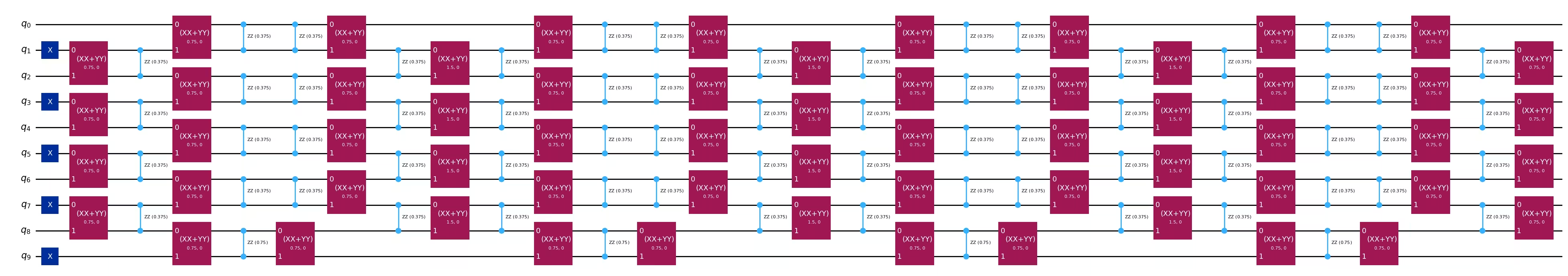
Kemudian kita membuat Circuit yang mengimplementasikan aproksimasi evolusi waktu Trotter.

from qiskit.synthesis import SuzukiTrotter
from qiskit_addon_utils.problem_generators import (
    generate_time_evolution_circuit,
)
from qiskit import QuantumCircuit

# Initial Neel state preparation
initial_state_circ = QuantumCircuit(L)
initial_state_circ.x([i for i in range(L) if i % 2 != 0])

all_circs = []
for total_time in trotter_times:
    mpf_trotter_circs = [
        generate_time_evolution_circuit(
            hamiltonian,
            time=total_time,
            synthesis=SuzukiTrotter(reps=num_steps, order=order),
        )
        for num_steps in mpf_trotter_steps
    ]

    mpf_trotter_circs = pm.run(
        mpf_trotter_circs
    )  # Collect XX and YY into XX + YY

    mpf_circuits = [
        initial_state_circ.compose(circuit) for circuit in mpf_trotter_circs
    ]
    all_circs.append(mpf_circuits)

mpf_circuits[-1].draw("mpl", fold=-1)

Selanjutnya, kita menghitung nilai ekspektasi terevolvsi-waktu dari Circuit Trotter.

from copy import deepcopy
from qiskit_aer import AerSimulator
from qiskit_ibm_runtime import EstimatorV2 as Estimator
from qiskit.transpiler.preset_passmanagers import generate_preset_pass_manager

aer_sim = AerSimulator()
estimator = Estimator(mode=aer_sim)

mpf_expvals_all_times, mpf_stds_all_times = [], []
for t, mpf_circuits in zip(trotter_times, all_circs):
    mpf_expvals = []
    circuits = [deepcopy(circuit) for circuit in mpf_circuits]
    pm_sim = generate_preset_pass_manager(
        backend=aer_sim, optimization_level=3
    )
    isa_circuits = pm_sim.run(circuits)
    result = estimator.run(
        [(circuit, observable) for circuit in isa_circuits], precision=0.005
    ).result()
    mpf_expvals = [res.data.evs for res in result]
    mpf_stds = [res.data.stds for res in result]
    mpf_expvals_all_times.append(mpf_expvals)
    mpf_stds_all_times.append(mpf_stds)

Kita juga menghitung nilai ekspektasi eksak untuk perbandingan.

from scipy.linalg import expm
from qiskit.quantum_info import Statevector

exact_expvals = []
for t in exact_evolution_times:
    # Exact expectation values
    exp_H = expm(-1j * t * hamiltonian.to_matrix())
    initial_state = Statevector(initial_state_circ).data
    time_evolved_state = exp_H @ initial_state

    exact_obs = (
        time_evolved_state.conj()
        @ observable.to_matrix()
        @ time_evolved_state
    ).real
    exact_expvals.append(exact_obs)

Koefisien MPF statis

MPF statis adalah yang nilai $x_j$-nya tidak bergantung pada waktu evolusi, $t$. Mari kita pertimbangkan PF orde $\chi = 1$ dengan $k_j$ langkah Trotter, yang bisa ditulis sebagai:

$S_1^{k_j}\left( \frac{t}{k_j} \right)=e^{-i H t}+ \sum_{n=1}^{\infty} A_n \frac{t^{n+1}}{k_j^n}$

di mana $A_n$ adalah matriks yang bergantung pada komutator suku $F_a$ dalam dekomposisi Hamiltonian. Penting untuk dicatat bahwa $A_n$ sendiri tidak bergantung pada waktu dan jumlah langkah Trotter $k_j$. Oleh karena itu, dimungkinkan untuk menghilangkan suku kesalahan orde rendah yang berkontribusi pada $\mu(t)$ dengan pemilihan bobot $x_j$ yang tepat dari kombinasi linear. Untuk menghilangkan kesalahan Trotter pada $l-1$ suku pertama (ini akan memberikan kontribusi terbesar karena sesuai dengan jumlah langkah Trotter yang lebih kecil) dalam ekspresi untuk $\mu(t)$, koefisien $x_j$ harus memenuhi persamaan berikut:

$\sum_{j=1}^l x_j = 1$ $\sum_{j=1}^{l-1} \frac{x_j}{k_j^{n}} = 0$

dengan $n=0, ... l-2$. Persamaan pertama menjamin tidak ada bias dalam keadaan $\mu(t)$ yang dikonstruksi, sementara persamaan kedua memastikan pembatalan kesalahan Trotter. Untuk PF orde lebih tinggi, persamaan kedua menjadi $\sum_{j=1}^{l-1} \frac{x_j}{k_j^{\eta}} = 0$ di mana $\eta = \chi + 2n$ untuk PF simetrik dan $\eta = \chi + n$ sebaliknya, dengan $n=0, ..., l-2$. Kesalahan yang dihasilkan (Ref. [1],[2]) adalah

$\epsilon = \mathcal{O} \left( \frac{t^{l+1}}{k_1^l} \right).$

Menentukan koefisien MPF statis untuk sekumpulan nilai $k_j$ tertentu berarti menyelesaikan sistem persamaan linear yang didefinisikan oleh dua persamaan di atas untuk variabel $x_j$: $Ax=b$. Di mana $x$ adalah koefisien yang kita cari, $A$ adalah matriks yang bergantung pada $k_j$ dan tipe PF yang kita gunakan ($S$), dan $b$ adalah vektor kendala. Secara spesifik:

$A_{0,j} = 1$ $A_{i>0,j} = k_{j}^{-(\chi + s(i-1))}$ $b_0 = 1$ $b_{i>0} = 0$

di mana $\chi$ adalah order, $s$ adalah $2$ jika symmetric bernilai True dan $1$ sebaliknya, $k_{j}$ adalah trotter_steps, dan $x$ adalah variabel yang dicari. Indeks $i$ dan $j$ dimulai dari $0$. Kita juga bisa memvisualisasikan ini dalam bentuk matriks:

$$A = \begin{bmatrix} A_{0,0} & A_{0,1} & A_{0,2} & ... \\ A_{1,0} & A_{1,1} & A_{1,2} & ... \\ A_{2,0} & A_{2,1} & A_{2,2} & ... \\ ... & ... & ... & ... \end{bmatrix} = \begin{bmatrix} 1 & 1 & 1 & ... \\ k_{0}^{-(\chi + s(1-1))} & k_{1}^{-(\chi + s(1-1))} & k_{2}^{-(\chi + s(1-1))} & ... \\ k_{0}^{-(\chi + s(2-1))} & k_{1}^{-(\chi + s(2-1))} & k_{2}^{-(\chi + s(2-1))} & ... \\ ... & ... & ... & ... \end{bmatrix}$$

dan

$$b = \begin{bmatrix} b_{0} \\ b_{1} \\ b_{2} \\ ... \end{bmatrix} = \begin{bmatrix} 1 \\ 0 \\ 0 \\ ... \end{bmatrix}$$

Untuk detail lebih lanjut, lihat dokumentasi Sistem Persamaan Linear (LSE).

Kita bisa menemukan solusi untuk $x$ secara analitik sebagai $x = A^{-1}b$; lihat misalnya Ref. [1] atau [2]. Namun, solusi eksak ini bisa "ill-conditioned", menghasilkan norma L1 yang sangat besar dari koefisien kita, $x$, yang bisa menyebabkan performa MPF yang buruk. Sebagai alternatif, kita juga bisa memperoleh solusi aproksimasi yang meminimalkan norma L1 dari $x$ untuk mencoba mengoptimalkan perilaku MPF.

Siapkan LSE

Setelah memilih nilai $k_j$ kita, kita harus terlebih dahulu mengonstruksi LSE, $Ax=b$ seperti yang dijelaskan di atas. Matriks $A$ tidak hanya bergantung pada $k_j$ tetapi juga pilihan PF kita, khususnya order-nya. Selain itu, kamu mungkin perlu mempertimbangkan apakah PF simetrik atau tidak (lihat [1]) dengan mengatur symmetric=True/False. Namun, ini tidak diperlukan, seperti yang ditunjukkan oleh Ref. [2].

from qiskit_addon_mpf.static import setup_static_lse

lse = setup_static_lse(mpf_trotter_steps, order=order, symmetric=symmetric)

Mari kita telusuri nilai-nilai yang dipilih di atas untuk mengonstruksi matriks $A$ dan vektor $b$. Dengan $j=0,1, 2$ langkah Trotter $k_j = [1, 2, 4]$, orde $\chi = 2$ dan pilihan langkah Trotter non-simetrik ($s=1$), kita punya elemen matriks $A$ di bawah baris pertama yang ditentukan oleh ekspresi $A_{i>0,j} = k_{j}^{-(2 + 1(i-1))}$, secara spesifik:

$A_{0,0} = A_{0,1} = A_{0,2} = 1$ $A_{1,j} = k_{j}^{-1} \rightarrow A_{1,0} = \frac{1}{1^2}, \;, A_{1,1} = \frac{1}{2^2}, \;, A_{1,2} = \frac{1}{4^2}$ $A_{2,j} = k_{j}^{-2} \rightarrow A_{2,0} = \frac{1}{1^3}, \;, A_{2,1} = \frac{1}{2^3}, \;, A_{2,2} = \frac{1}{4^3}$

atau dalam bentuk matriks:

$$A = \begin{bmatrix} 1 & 1 & 1\\ 1 & \frac{1}{2^2} & \frac{1}{4^2} \\ 1 & \frac{1}{2^3} & \frac{1}{4^3} \\ \end{bmatrix}$$

Ini bisa dilihat dengan memeriksa objek lse:

lse.A

array([[1.      , 1.      , 1.      ],
       [1.      , 0.25    , 0.0625  ],
       [1.      , 0.125   , 0.015625]])

Sementara vektor kendala $b$ memiliki elemen berikut: $b_{0} = 1$ $b_1 = b_2 = 0$

Jadi,

$$b = \begin{bmatrix} 1 \\ 0 \\ 0 \end{bmatrix}$$

Dan serupa dalam lse:

lse.b

array([1., 0., 0.])

Objek lse memiliki metode untuk menemukan koefisien statis $x_j$ yang memenuhi sistem persamaan.

mpf_coeffs = lse.solve()
print(
    f"The static coefficients associated with the ansatze are: {mpf_coeffs}"
)

The static coefficients associated with the ansatze are: [ 0.04761905 -0.57142857  1.52380952]

Optimalkan $x$ menggunakan model eksak

Sebagai alternatif dari komputasi $x=A^{-1}b$, kamu juga bisa menggunakan setup_exact_model untuk mengonstruksi instance cvxpy.Problem yang menggunakan LSE sebagai kendala dan solusi optimalnya akan menghasilkan $x$.

Di bagian selanjutnya, akan jelas mengapa antarmuka ini ada.

from qiskit_addon_mpf.costs import setup_exact_problem

model_exact, coeffs_exact = setup_exact_problem(lse)
model_exact.solve()
print(coeffs_exact.value)

[ 0.04761905 -0.57142857  1.52380952]

Sebagai indikator apakah MPF yang dikonstruksi dengan koefisien ini akan menghasilkan hasil yang baik, kita bisa menggunakan norma L1 (lihat juga Ref. [1]).

print(
    "L1 norm of the exact coefficients:",
    np.linalg.norm(coeffs_exact.value, ord=1),
)  # ord specifies the norm. ord=1 is for L1

L1 norm of the exact coefficients: 2.1428571428556378

Optimalkan $x$ menggunakan model aproksimasi

Mungkin terjadi bahwa norma L1 untuk sekumpulan nilai $k_j$ yang dipilih dianggap terlalu tinggi. Jika itu terjadi dan kamu tidak bisa memilih sekumpulan nilai $k_j$ yang berbeda, kamu bisa menggunakan solusi aproksimasi untuk LSE alih-alih yang eksak.

Untuk melakukannya, cukup gunakan setup_approximate_model untuk mengonstruksi instance cvxpy.Problem yang berbeda, yang membatasi norma L1 ke ambang batas yang dipilih sambil meminimalkan selisih antara $Ax$ dan $b$.

from qiskit_addon_mpf.costs import setup_sum_of_squares_problem

model_approx, coeffs_approx = setup_sum_of_squares_problem(
    lse, max_l1_norm=1.5
)
model_approx.solve()
print(coeffs_approx.value)
print(
    "L1 norm of the approximate coefficients:",
    np.linalg.norm(coeffs_approx.value, ord=1),
)

[-1.10294118e-03 -2.48897059e-01  1.25000000e+00]
L1 norm of the approximate coefficients: 1.5

Perlu dicatat bahwa kamu punya kebebasan penuh dalam cara menyelesaikan masalah optimasi ini, yang berarti kamu bisa mengubah solver optimasi, ambang batas konvergensinya, dan sebagainya. Lihat panduan masing-masing tentang Cara menggunakan model aproksimasi.

Koefisien MPF dinamis

Di bagian sebelumnya, kita memperkenalkan MPF statis yang memperbaiki aproksimasi Trotter standar. Namun, versi statis ini belum tentu meminimalkan kesalahan aproksimasi. Lebih konkretnya, MPF statis, yang dilambangkan $\mu^S(t)$, bukanlah proyeksi optimal dari $\rho(t)$ ke subruang yang direntang oleh state-state formula produk $\{\rho_{k_i}(t)\}_{i=1}^r$.

Untuk mengatasi ini, kita mempertimbangkan MPF dinamis (diperkenalkan dalam Ref. [2] dan didemonstrasikan secara eksperimental dalam Ref. [3]) yang memang meminimalkan kesalahan aproksimasi dalam norma Frobenius. Secara formal, kita fokus pada minimasi

$$\|\rho(t) - \mu^D(t)\|_F^2 \;=\; \mathrm{Tr}\bigl[ \left( \rho(t) - \mu^D(t)\right)^2 \bigr],$$

terhadap beberapa koefisien $x_i(t)$ pada setiap waktu $t$. Proyektor optimal dalam norma Frobenius kemudian adalah $\mu^D(t) \;=\; \sum_{i=1}^r x_i(t)\,\rho_{k_i}(t)$, dan kita sebut $\mu^D(t)$ sebagai MPF dinamis. Dengan mensubstitusi definisi di atas:

$$\|\rho(t) - \mu^D(t)\|_F^2 \;=\; \\ = \mathrm{Tr}\bigl[ \left( \rho(t) - \mu^D(t)\right)^2 \bigr] \;=\; \\ = \mathrm{Tr}\bigl[ \left( \rho(t) - \sum_{i=1}^r x_i(t)\,\rho_{k_i}(t) \right) \left( \rho(t) - \sum_{j=1}^r x_j(t)\,\rho_{k_j}(t) \right) \bigr] \;=\; \\ = 1 \;+\; \sum_{i,j=1}^r M_{i,j}(t)\,x_i(t)\,x_j(t) \;-\; 2 \sum_{i=1}^r L_i^{\mathrm{exact}}(t)\,x_i(t),$$

di mana $M_{i,j}(t)$ adalah matriks Gram, yang didefinisikan oleh

$$M_{i,j}(t) \;=\; \mathrm{Tr}\bigl[\rho_{k_i}(t)\,\rho_{k_j}(t)\bigr] \;=\; \bigl|\langle \psi_{\mathrm{in}} \!\mid S\bigl(t/k_i\bigr)^{-k_i}\,S\bigl(t/k_j\bigr)^{k_j} \!\mid \psi_{\mathrm{in}} \rangle \bigr|^2.$$

dan

$$L_i^{\mathrm{exact}}(t) = \mathrm{Tr}[\rho(t)\,\rho_{k_i}(t)]$$

merepresentasikan tumpang tindih antara state eksak $\rho(t)$ dan setiap aproksimasi formula produk $\rho_{k_i}(t)$. Dalam skenario praktis, tumpang tindih ini hanya bisa diukur secara aproksimasi karena noise atau akses parsial ke $\rho(t)$.

Di sini, $\lvert\psi_{\mathrm{in}}\rangle$ adalah state awal, dan $S(\cdot)$ adalah operasi yang diterapkan dalam formula produk. Dengan memilih koefisien $x_i(t)$ yang meminimalkan ekspresi ini (dan menangani data tumpang tindih yang aproksimasi ketika $\rho(t)$ tidak sepenuhnya diketahui), kita mendapatkan aproksimasi dinamis "terbaik" (dalam arti norma Frobenius) dari $\rho(t)$ dalam subruang MPF. Kuantitas $L_i(t)$ dan $M_{i,j}(t)$ bisa dihitung secara efisien menggunakan metode tensor network [3]. Addon Qiskit MPF menyediakan beberapa "backend" untuk melakukan perhitungan ini. Contoh di bawah menunjukkan cara paling fleksibel untuk melakukannya, dan dokumentasi backend berbasis lapisan TeNPy juga menjelaskannya secara detail. Untuk menggunakan metode ini, mulailah dari Circuit yang mengimplementasikan evolusi waktu yang diinginkan dan buat model-model yang merepresentasikan operasi-operasi ini dari lapisan-lapisan Circuit yang bersangkutan. Terakhir, sebuah objek Evolver dibuat yang bisa digunakan untuk menghasilkan kuantitas yang berevolusi dalam waktu $M_{i,j}(t)$ dan $L_i(t)$. Kita mulai dengan membuat objek Evolver yang berkorespondensi dengan evolusi waktu aproksimasi (ApproxEvolverFactory) yang diimplementasikan oleh Circuit-Circuit. Khususnya, perhatikan baik-baik variabel order agar sesuai. Perlu dicatat bahwa dalam menghasilkan Circuit-Circuit yang berkorespondensi dengan evolusi waktu aproksimasi, kita menggunakan nilai placeholder untuk time = 1.0 dan jumlah langkah Trotter (reps=1). Circuit-Circuit aproksimasi yang benar kemudian dihasilkan oleh solver masalah dinamis di setup_dynamic_lse.

from qiskit_addon_utils.slicing import slice_by_depth
from qiskit_addon_mpf.backends.tenpy_layers import LayerModel
from qiskit_addon_mpf.backends.tenpy_layers import LayerwiseEvolver
from functools import partial

# Create approximate time-evolution circuits
single_2nd_order_circ = generate_time_evolution_circuit(
    hamiltonian, time=1.0, synthesis=SuzukiTrotter(reps=1, order=order)
)
single_2nd_order_circ = pm.run(single_2nd_order_circ)  # collect XX and YY

# Find layers in the circuit
layers = slice_by_depth(single_2nd_order_circ, max_slice_depth=1)

# Create tensor network models
models = [
    LayerModel.from_quantum_circuit(layer, conserve="Sz") for layer in layers
]

# Create the time-evolution object
approx_factory = partial(
    LayerwiseEvolver,
    layers=models,
    options={
        "preserve_norm": False,
        "trunc_params": {
            "chi_max": 64,
            "svd_min": 1e-8,
            "trunc_cut": None,
        },
        "max_delta_t": 2,
    },
)

peringatan

Opsi-opsi LayerwiseEvolver yang menentukan detail simulasi tensor network harus dipilih dengan hati-hati untuk menghindari pembentukan masalah optimasi yang tidak terdefinisi dengan baik.

Kemudian kita menyiapkan evolver eksak (misalnya, ExactEvolverFactory), yang mengembalikan objek Evolver yang menghitung evolusi waktu sejati atau "referensi". Secara realistis, kita akan mengaproksimasi evolusi eksak dengan menggunakan formula Suzuki–Trotter orde lebih tinggi atau metode andal lainnya dengan langkah waktu kecil. Di bawah ini, kita mengaproksimasi state yang berevolusi dalam waktu eksak dengan formula Suzuki-Trotter orde empat menggunakan langkah waktu kecil dt=0.1, yang berarti jumlah langkah Trotter yang digunakan pada waktu $t$ adalah $k=t/dt$. Kita juga menentukan beberapa opsi truncation spesifik TeNPy untuk membatasi dimensi bond maksimum dari tensor network yang mendasarinya, serta nilai singular minimum dari bond tensor network yang dipisah. Parameter-parameter ini bisa mempengaruhi akurasi nilai ekspektasi yang dihitung dengan koefisien MPF dinamis, sehingga penting untuk mengeksplorasi berbagai nilai untuk menemukan keseimbangan optimal antara waktu komputasi dan akurasi. Perlu dicatat bahwa perhitungan koefisien MPF tidak bergantung pada nilai ekspektasi PF yang diperoleh dari eksekusi hardware, sehingga bisa diatur dalam post-processing.

single_4th_order_circ = generate_time_evolution_circuit(
    hamiltonian, time=1.0, synthesis=SuzukiTrotter(reps=1, order=4)
)
single_4th_order_circ = pm.run(single_4th_order_circ)
exact_model_layers = [
    LayerModel.from_quantum_circuit(layer, conserve="Sz")
    for layer in slice_by_depth(single_4th_order_circ, max_slice_depth=1)
]

exact_factory = partial(
    LayerwiseEvolver,
    layers=exact_model_layers,
    dt=0.1,
    options={
        "preserve_norm": False,
        "trunc_params": {
            "chi_max": 64,
            "svd_min": 1e-8,
            "trunc_cut": None,
        },
        "max_delta_t": 2,
    },
)

Selanjutnya, buat state awal sistem dalam format yang kompatibel dengan TeNPy (misalnya, MPS_neel_state=$\vert 0101...01 \rangle$). Ini menyiapkan fungsi gelombang many-body yang akan kita evolusikan dalam waktu $\lvert\psi_{\mathrm{in}}\rangle$ sebagai sebuah tensor.

from qiskit_addon_mpf.backends.tenpy_tebd import MPOState
from qiskit_addon_mpf.backends.tenpy_tebd import MPS_neel_state

def identity_factory():
    return MPOState.initialize_from_lattice(models[0].lat, conserve=True)

mps_initial_state = MPS_neel_state(models[0].lat)

Untuk setiap langkah waktu $t$, kita menyiapkan sistem persamaan linear dinamis dengan metode setup_dynamic_lse. Objek yang bersangkutan berisi informasi tentang masalah MPF dinamis: lse.A memberikan matriks Gram $M$ sementara lse.b memberikan tumpang tindih $L$. Kita kemudian bisa menyelesaikan LSE (jika tidak terdefinisi dengan baik) untuk menemukan koefisien dinamis menggunakan setup_frobenius_problem. Penting untuk dicatat perbedaan dengan koefisien statis, yang hanya bergantung pada detail formula produk yang digunakan dan tidak bergantung pada detail evolusi waktu (Hamiltonian dan state awal).

from qiskit_addon_mpf.dynamic import setup_dynamic_lse
from qiskit_addon_mpf.costs import setup_frobenius_problem

mpf_dynamic_coeffs_list = []
for t in trotter_times:
    print(f"Computing dynamic coefficients for time={t}")
    lse = setup_dynamic_lse(
        mpf_trotter_steps,
        t,
        identity_factory,
        exact_factory,
        approx_factory,
        mps_initial_state,
    )
    problem, coeffs = setup_frobenius_problem(lse)
    try:
        problem.solve()
        mpf_dynamic_coeffs_list.append(coeffs.value)
    except Exception as error:
        mpf_dynamic_coeffs_list.append(np.zeros(len(mpf_trotter_steps)))
        print(error, "Calculation Failed for time", t)
    print("")

Computing dynamic coefficients for time=0.5

Computing dynamic coefficients for time=0.6

Computing dynamic coefficients for time=0.7

Computing dynamic coefficients for time=0.7999999999999999

Computing dynamic coefficients for time=0.8999999999999999

Computing dynamic coefficients for time=0.9999999999999999

Computing dynamic coefficients for time=1.0999999999999999

Computing dynamic coefficients for time=1.1999999999999997

Computing dynamic coefficients for time=1.2999999999999998

Computing dynamic coefficients for time=1.4

Computing dynamic coefficients for time=1.4999999999999998

Terakhir, plot nilai-nilai ekspektasi ini sepanjang waktu evolusi.

import matplotlib.pyplot as plt

sym = {1: "^", 2: "s", 4: "p"}
# Get expectation values at all times for each Trotter step
for k, step in enumerate(mpf_trotter_steps):
    trotter_curve, trotter_curve_error = [], []
    for trotter_expvals, trotter_stds in zip(
        mpf_expvals_all_times, mpf_stds_all_times
    ):
        trotter_curve.append(trotter_expvals[k])
        trotter_curve_error.append(trotter_stds[k])

    plt.errorbar(
        trotter_times,
        trotter_curve,
        yerr=trotter_curve_error,
        alpha=0.5,
        markersize=4,
        marker=sym[step],
        color="grey",
        label=f"{mpf_trotter_steps[k]} Trotter steps",
    )  # , , )

# Get expectation values at all times for the static MPF with exact coeffs
exact_mpf_curve, exact_mpf_curve_error = [], []
for trotter_expvals, trotter_stds in zip(
    mpf_expvals_all_times, mpf_stds_all_times
):
    mpf_std = np.sqrt(
        sum(
            [
                (coeff**2) * (std**2)
                for coeff, std in zip(coeffs_exact.value, trotter_stds)
            ]
        )
    )
    exact_mpf_curve_error.append(mpf_std)
    exact_mpf_curve.append(trotter_expvals @ coeffs_exact.value)

plt.errorbar(
    trotter_times,
    exact_mpf_curve,
    yerr=exact_mpf_curve_error,
    markersize=4,
    marker="o",
    label="Static MPF - Exact",
    color="purple",
)

# Get expectation values at all times for the static MPF with approximate
approx_mpf_curve, approx_mpf_curve_error = [], []
for trotter_expvals, trotter_stds in zip(
    mpf_expvals_all_times, mpf_stds_all_times
):
    mpf_std = np.sqrt(
        sum(
            [
                (coeff**2) * (std**2)
                for coeff, std in zip(coeffs_approx.value, trotter_stds)
            ]
        )
    )
    approx_mpf_curve_error.append(mpf_std)
    approx_mpf_curve.append(trotter_expvals @ coeffs_approx.value)

plt.errorbar(
    trotter_times,
    approx_mpf_curve,
    yerr=approx_mpf_curve_error,
    markersize=4,
    marker="o",
    color="orange",
    label="Static MPF - Approximate",
)

# # Get expectation values at all times for the dynamic MPF
dynamic_mpf_curve, dynamic_mpf_curve_error = [], []
for trotter_expvals, trotter_stds, dynamic_coeffs in zip(
    mpf_expvals_all_times, mpf_stds_all_times, mpf_dynamic_coeffs_list
):
    mpf_std = np.sqrt(
        sum(
            [
                (coeff**2) * (std**2)
                for coeff, std in zip(dynamic_coeffs, trotter_stds)
            ]
        )
    )
    dynamic_mpf_curve_error.append(mpf_std)
    dynamic_mpf_curve.append(trotter_expvals @ dynamic_coeffs)

plt.errorbar(
    trotter_times,
    dynamic_mpf_curve,
    yerr=dynamic_mpf_curve_error,
    markersize=4,
    marker="o",
    color="pink",
    label="Dynamic MPF",
)

plt.plot(
    exact_evolution_times,
    exact_expvals,
    lw=3,
    color="red",
    label="Exact time-evolution",
)

plt.title(
    f"Expectation values for (ZZ,{(L//2-1, L//2)}) as a function of time"
)
plt.xlabel("Time")
plt.ylabel("Expectation Value")
plt.legend()
plt.grid()

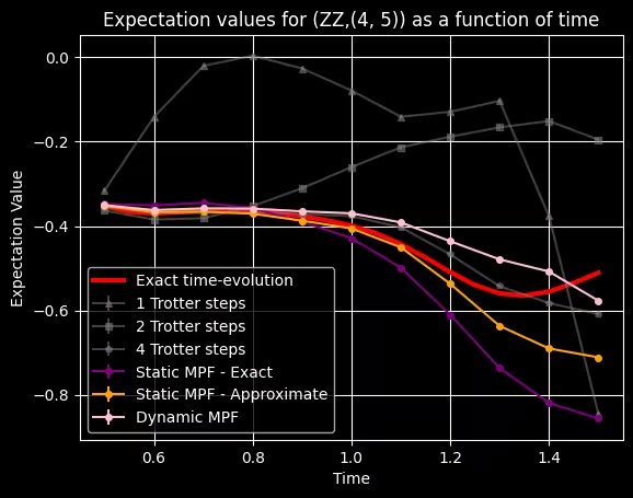
Dalam kasus seperti contoh di atas, di mana PF $k=1$ berperilaku buruk di semua waktu, kualitas hasil MPF dinamis juga sangat terpengaruh. Dalam situasi seperti ini, berguna untuk menginvestigasi kemungkinan penggunaan PF individual dengan jumlah langkah Trotter yang lebih tinggi untuk meningkatkan kualitas hasil secara keseluruhan. Dalam simulasi-simulasi ini, kita melihat interaksi berbagai jenis kesalahan: kesalahan dari sampling terbatas, dan kesalahan Trotter dari formula produk. MPF membantu mengurangi kesalahan Trotter akibat formula produk tetapi mengakibatkan kesalahan sampling yang lebih tinggi dibandingkan formula produk. Ini bisa menguntungkan, karena formula produk dapat mengurangi kesalahan sampling dengan peningkatan sampling, tetapi kesalahan sistematis akibat aproksimasi Trotter tetap tidak tersentuh.

Perilaku menarik lainnya yang bisa kita amati dari plot adalah bahwa nilai ekspektasi untuk PF dengan $k=1$ mulai berperilaku erratik (di samping tidak menjadi aproksimasi yang baik untuk yang eksak) pada waktu-waktu di mana $t/k > 1$, seperti yang dijelaskan dalam panduan tentang cara memilih jumlah langkah Trotter.

Langkah 1: Petakan input klasik ke masalah kuantum

Sekarang kita pertimbangkan satu waktu $t=1.0$ dan hitung nilai ekspektasi magnetisasi dengan berbagai metode menggunakan satu QPU. Pilihan $t$ yang khusus ini dilakukan untuk memaksimalkan perbedaan antara berbagai metode dan mengamati efektivitas relatifnya. Untuk menentukan jendela waktu di mana MPF dinamis dijamin menghasilkan besaran yang dapat diamati dengan kesalahan lebih rendah dari semua formula Trotter individual dalam multi-product, kita bisa mengimplementasikan "MPF test" - lihat persamaan (17) dan teks sekitarnya dalam [3].

Siapkan Circuit-Circuit Trotter

Pada titik ini, kita sudah menemukan koefisien ekspansi, $x$, dan yang tersisa hanyalah menghasilkan Circuit-Circuit kuantum yang di-Trotterize. Sekali lagi, modul qiskit_addon_utils.problem_generators hadir dengan fungsi yang berguna untuk melakukan ini:

from qiskit.synthesis import SuzukiTrotter
from qiskit_addon_utils.problem_generators import (
    generate_time_evolution_circuit,
)
from qiskit import QuantumCircuit

total_time = 1.0
mpf_circuits = []
for k in mpf_trotter_steps:
    # Initial Neel state preparation
    circuit = QuantumCircuit(L)
    circuit.x([i for i in range(L) if i % 2 != 0])

    trotter_circ = generate_time_evolution_circuit(
        hamiltonian,
        synthesis=SuzukiTrotter(order=order, reps=k),
        time=total_time,
    )

    circuit.compose(trotter_circ, inplace=True)

    mpf_circuits.append(pm.run(circuit))

mpf_circuits[-1].draw("mpl", fold=-1, scale=0.4)

Langkah 2: Optimalkan masalah untuk eksekusi hardware kuantum

Mari kita kembali ke perhitungan nilai ekspektasi untuk satu titik waktu. Kita akan memilih Backend untuk menjalankan eksperimen di hardware.

from qiskit_ibm_runtime import QiskitRuntimeService

service = QiskitRuntimeService()
backend = service.least_busy(min_num_qubits=127)
print(backend)

qubits = list(range(backend.num_qubits))

Kemudian kita menghapus qubit-qubit outlier dari coupling map untuk memastikan bahwa tahap layout Transpiler tidak menyertakannya. Di bawah ini kita menggunakan properti Backend yang dilaporkan yang tersimpan dalam objek target dan menghapus qubit-qubit yang memiliki kesalahan pengukuran atau gate dua-qubit di atas ambang batas tertentu (max_meas_err, max_twoq_err) atau waktu $T_2$ (yang menentukan kehilangan koherensi) di bawah ambang batas tertentu (min_t2).

import copy
from qiskit.transpiler import Target, CouplingMap

target = backend.target
instruction_2q = "cz"

cmap = target.build_coupling_map(filter_idle_qubits=True)
cmap_list = list(cmap.get_edges())

max_meas_err = 0.012
min_t2 = 40
max_twoq_err = 0.005

# Remove qubits with bad measurement or t2
cust_cmap_list = copy.deepcopy(cmap_list)
for q in range(target.num_qubits):
    meas_err = target["measure"][(q,)].error
    if target.qubit_properties[q].t2 is not None:
        t2 = target.qubit_properties[q].t2 * 1e6
    else:
        t2 = 0
    if meas_err > max_meas_err or t2 < min_t2:
        # print(q)
        for q_pair in cmap_list:
            if q in q_pair:
                try:
                    cust_cmap_list.remove(q_pair)
                except ValueError:
                    continue

# Remove qubits with bad 2q gate or t2
for q in cmap_list:
    twoq_gate_err = target[instruction_2q][q].error
    if twoq_gate_err > max_twoq_err:
        # print(q)
        for q_pair in cmap_list:
            if q == q_pair:
                try:
                    cust_cmap_list.remove(q_pair)
                except ValueError:
                    continue

cust_cmap = CouplingMap(cust_cmap_list)

cust_target = Target.from_configuration(
    basis_gates=backend.configuration().basis_gates
    + ["measure"],  # or whatever new set of gates
    coupling_map=cust_cmap,
)

sorted_components = sorted(
    [list(comp.physical_qubits) for comp in cust_cmap.connected_components()],
    reverse=True,
)
print("size of largest component", len(sorted_components[0]))

size of largest component 10

Kita perlu mengatur max_meas_err, min_t2, dan max_twoq_err sedemikian rupa sehingga kita menemukan subset qubit yang cukup besar untuk mendukung Circuit yang akan dijalankan. Dalam kasus kita, cukup dengan menemukan rantai 1D 10-qubit.

cust_cmap.draw()

Kita kemudian bisa memetakan Circuit dan besaran yang dapat diamati ke qubit-qubit fisik perangkat.

from qiskit.transpiler.preset_passmanagers import generate_preset_pass_manager

transpiler = generate_preset_pass_manager(
    optimization_level=3, target=cust_target
)

transpiled_circuits = [transpiler.run(circ) for circ in mpf_circuits]

qubits_layouts = [
    [
        idx
        for idx, qb in circuit.layout.initial_layout.get_physical_bits().items()
        if qb._register.name != "ancilla"
    ]
    for circuit in transpiled_circuits
]

transpiled_circuits = []
for circuit, layout in zip(mpf_circuits, qubits_layouts):
    transpiler = generate_preset_pass_manager(
        optimization_level=3, backend=backend, initial_layout=layout
    )
    transpiled_circuit = transpiler.run(circuit)
    transpiled_circuits.append(transpiled_circuit)

# transform the observable defined on virtual qubits to
# an observable defined on all physical qubits
isa_observables = [
    observable.apply_layout(circ.layout) for circ in transpiled_circuits
]

print(transpiled_circuits[-1].depth(lambda x: x.operation.num_qubits == 2))
print(transpiled_circuits[-1].count_ops())
transpiled_circuits[-1].draw("mpl", idle_wires=False, fold=False)

51
OrderedDict([('sx', 310), ('rz', 232), ('cz', 132), ('x', 19)])

Langkah 3: Eksekusi menggunakan primitif Qiskit

Dengan primitif Estimator kita bisa mendapatkan estimasi nilai ekspektasi dari QPU. Kita menjalankan circuit AQC yang sudah dioptimalkan dengan teknik mitigasi dan supresi error tambahan.

from qiskit_ibm_runtime import EstimatorV2 as Estimator

estimator = Estimator(mode=backend)
estimator.options.default_shots = 30000

# Set simple error suppression/mitigation options
estimator.options.dynamical_decoupling.enable = True
estimator.options.twirling.enable_gates = True
estimator.options.twirling.enable_measure = True
estimator.options.twirling.num_randomizations = "auto"
estimator.options.twirling.strategy = "active-accum"
estimator.options.resilience.measure_mitigation = True
estimator.options.experimental.execution_path = "gen3-turbo"

estimator.options.resilience.zne_mitigation = True
estimator.options.resilience.zne.noise_factors = (1, 3, 5)
estimator.options.resilience.zne.extrapolator = ("exponential", "linear")

estimator.options.environment.job_tags = ["mpf small"]

job = estimator.run(
    [
        (circ, observable)
        for circ, observable in zip(transpiled_circuits, isa_observables)
    ]
)

Langkah 4: Pasca-proses dan kembalikan hasil dalam format klasik yang diinginkan

Satu-satunya langkah pasca-proses adalah menggabungkan nilai ekspektasi yang diperoleh dari primitif Qiskit Runtime pada berbagai langkah Trotter menggunakan koefisien MPF yang sesuai. Untuk suatu observable $A$ kita punya:

$\langle A \rangle_{\text{mpf}} = \text{Tr} [A \mu(t)] = \sum_{j} x_j \text{Tr} [A \rho_{k_j}] = \sum_{j} x_j \langle A \rangle_j$

Pertama, kita ekstrak nilai ekspektasi individual yang diperoleh untuk masing-masing circuit Trotter:

result_exp = job.result()
evs_exp = [res.data.evs for res in result_exp]
evs_std = [res.data.stds for res in result_exp]

print(evs_exp)

[array(-0.06361607), array(-0.23820448), array(-0.50271805)]

Selanjutnya, kita cukup menggabungkannya kembali dengan koefisien MPF kita untuk menghasilkan nilai ekspektasi total dari MPF. Di bawah ini kita melakukannya untuk setiap cara berbeda yang telah kita gunakan untuk menghitung $x$.

exact_mpf_std = np.sqrt(
    sum(
        [
            (coeff**2) * (std**2)
            for coeff, std in zip(coeffs_exact.value, evs_std)
        ]
    )
)
print(
    "Exact static MPF expectation value: ",
    evs_exp @ coeffs_exact.value,
    "+-",
    exact_mpf_std,
)
approx_mpf_std = np.sqrt(
    sum(
        [
            (coeff**2) * (std**2)
            for coeff, std in zip(coeffs_approx.value, evs_std)
        ]
    )
)
print(
    "Approximate static MPF expectation value: ",
    evs_exp @ coeffs_approx.value,
    "+-",
    approx_mpf_std,
)
dynamic_mpf_std = np.sqrt(
    sum(
        [
            (coeff**2) * (std**2)
            for coeff, std in zip(mpf_dynamic_coeffs_list[7], evs_std)
        ]
    )
)
print(
    "Dynamic MPF expectation value: ",
    evs_exp @ mpf_dynamic_coeffs_list[7],
    "+-",
    dynamic_mpf_std,
)

Exact static MPF expectation value:  -0.6329590442738475 +- 0.012798249760406036
Approximate static MPF expectation value:  -0.5690390035339492 +- 0.010459559917168473
Dynamic MPF expectation value:  -0.4655579758795695 +- 0.007639139186720507

Terakhir, untuk masalah kecil ini kita bisa menghitung nilai referensi eksak menggunakan scipy.linalg.expm sebagai berikut:

from scipy.linalg import expm
from qiskit.quantum_info import Statevector

exp_H = expm(-1j * total_time * hamiltonian.to_matrix())

initial_state_circuit = QuantumCircuit(L)
initial_state_circuit.x([i for i in range(L) if i % 2 != 0])
initial_state = Statevector(initial_state_circuit).data

time_evolved_state = exp_H @ initial_state

exact_obs = (
    time_evolved_state.conj() @ observable.to_matrix() @ time_evolved_state
)
print("Exact expectation value ", exact_obs.real)

Exact expectation value  -0.39909900734489434

sym = {1: "^", 2: "s", 4: "p"}
# Get expectation values at all times for each Trotter step
for k, step in enumerate(mpf_trotter_steps):
    plt.errorbar(
        k,
        evs_exp[k],
        yerr=evs_std[k],
        alpha=0.5,
        markersize=4,
        marker=sym[step],
        color="grey",
        label=f"{mpf_trotter_steps[k]} Trotter steps",
    )  # , , )

plt.errorbar(
    3,
    evs_exp @ coeffs_exact.value,
    yerr=exact_mpf_std,
    markersize=4,
    marker="o",
    color="purple",
    label="Static MPF",
)

plt.errorbar(
    4,
    evs_exp @ coeffs_approx.value,
    yerr=approx_mpf_std,
    markersize=4,
    marker="o",
    color="orange",
    label="Approximate static MPF",
)

plt.errorbar(
    5,
    evs_exp @ mpf_dynamic_coeffs_list[7],
    yerr=dynamic_mpf_std,
    markersize=4,
    marker="o",
    color="pink",
    label="Dynamic MPF",
)

plt.axhline(
    y=exact_obs.real,
    linestyle="--",
    color="red",
    label="Exact time-evolution",
)

plt.title(
    f"Expectation values for (ZZ,{(L//2-1, L//2)}) at time {total_time} for the different methods "
)
plt.xlabel("Method")
plt.ylabel("Expectation Value")
plt.legend(loc="upper center", bbox_to_anchor=(0.5, -0.2), ncol=2)
plt.grid(alpha=0.1)
plt.tight_layout()
plt.show()

Pada contoh di atas, metode MPF dinamis menunjukkan performa terbaik dari segi nilai ekspektasi, melampaui apa yang akan kita dapatkan jika hanya menggunakan jumlah langkah Trotter tertinggi saja. Meskipun berbagai teknik MPF tidak selalu menghasilkan nilai ekspektasi yang lebih baik dibanding jumlah langkah Trotter tertinggi (seperti model eksak dan aproksimasi pada plot di atas), standar deviasi dari nilai-nilai tersebut dengan baik menangkap peningkatan variansi yang terjadi saat menggunakan teknik MPF. Ini menyoroti ketidakpastian seputar nilai ekspektasi yang diperoleh, yang selalu mencakup nilai ekspektasi yang kita harapkan dari evolusi waktu eksak sistem. Di sisi lain, nilai ekspektasi yang dihitung dengan jumlah langkah Trotter lebih rendah gagal menangkap nilai ekspektasi eksak dalam rentang ketidakpastiannya, sehingga secara yakin mengembalikan hasil yang salah.

def relative_error(ev, exact_ev):
    return abs(ev - exact_ev)

relative_error_k = [relative_error(ev, exact_obs.real) for ev in evs_exp]
relative_error_mpf = relative_error(evs_exp @ mpf_coeffs, exact_obs.real)
relative_error_approx_mpf = relative_error(
    evs_exp @ coeffs_approx.value, exact_obs.real
)
relative_error_dynamic_mpf = relative_error(
    evs_exp @ mpf_dynamic_coeffs_list[7], exact_obs.real
)

print("relative error for each trotter steps", relative_error_k)
print("relative error with MPF exact coeffs", relative_error_mpf)
print("relative error with MPF approx coeffs", relative_error_approx_mpf)
print("relative error with MPF dynamic coeffs", relative_error_dynamic_mpf)

relative error for each trotter steps [0.33548293650112293, 0.16089452939226306, 0.10361904247828346]
relative error with MPF exact coeffs 0.2338600369291003
relative error with MPF approx coeffs 0.16993999618905486
relative error with MPF dynamic coeffs 0.06645896853467514

Bagian II: perbesar skalanya

Mari kita perbesar skala masalahnya hingga melampaui apa yang bisa disimulasikan secara eksak. Di bagian ini kita akan fokus mereproduksi sebagian hasil yang ditampilkan di Ref. [3].

Langkah 1: Petakan input klasik ke masalah kuantum

Hamiltonian

Untuk contoh skala besar, kita menggunakan model XXZ pada barisan 50 situs:

$$\hat{\mathcal{H}}_{XXZ} = \sum_{i=1}^{L-1} J_{i,(i+1)}\left(X_i X_{(i+1)}+Y_i Y_{(i+1)}+ 2\cdot Z_i Z_{(i+1)} \right) \, ,$$

di mana $J_{i,(i+1)}$ adalah koefisien acak yang bersesuaian dengan tepi $(i, i+1)$. Ini adalah Hamiltonian yang dipertimbangkan dalam demonstrasi yang disajikan di Ref. [3].

L = 50
# Generate some coupling map to use for this example
coupling_map = CouplingMap.from_line(L, bidirectional=False)
graphviz_draw(coupling_map.graph, method="circo")

import numpy as np
from qiskit.quantum_info import SparsePauliOp, Pauli

# Generate random coefficients for our XXZ Hamiltonian
np.random.seed(0)
even_edges = list(coupling_map.get_edges())[::2]
odd_edges = list(coupling_map.get_edges())[1::2]

Js = np.random.uniform(0.5, 1.5, size=L)
hamiltonian = SparsePauliOp(Pauli("I" * L))
for i, edge in enumerate(even_edges + odd_edges):
    hamiltonian += SparsePauliOp.from_sparse_list(
        [
            ("XX", (edge), 2 * Js[i]),
            ("YY", (edge), 2 * Js[i]),
            ("ZZ", (edge), 4 * Js[i]),
        ],
        num_qubits=L,
    )

print(hamiltonian)

SparsePauliOp(['IIIIIIIIIIIIIIIIIIIIIIIIIIIIIIIIIIIIIIIIIIIIIIIIII', 'IIIIIIIIIIIIIIIIIIIIIIIIIIIIIIIIIIIIIIIIIIIIIIIIXX', 'IIIIIIIIIIIIIIIIIIIIIIIIIIIIIIIIIIIIIIIIIIIIIIIIYY', 'IIIIIIIIIIIIIIIIIIIIIIIIIIIIIIIIIIIIIIIIIIIIIIIIZZ', 'IIIIIIIIIIIIIIIIIIIIIIIIIIIIIIIIIIIIIIIIIIIIIIXXII', 'IIIIIIIIIIIIIIIIIIIIIIIIIIIIIIIIIIIIIIIIIIIIIIYYII', 'IIIIIIIIIIIIIIIIIIIIIIIIIIIIIIIIIIIIIIIIIIIIIIZZII', 'IIIIIIIIIIIIIIIIIIIIIIIIIIIIIIIIIIIIIIIIIIIIXXIIII', 'IIIIIIIIIIIIIIIIIIIIIIIIIIIIIIIIIIIIIIIIIIIIYYIIII', 'IIIIIIIIIIIIIIIIIIIIIIIIIIIIIIIIIIIIIIIIIIIIZZIIII', 'IIIIIIIIIIIIIIIIIIIIIIIIIIIIIIIIIIIIIIIIIIXXIIIIII', 'IIIIIIIIIIIIIIIIIIIIIIIIIIIIIIIIIIIIIIIIIIYYIIIIII', 'IIIIIIIIIIIIIIIIIIIIIIIIIIIIIIIIIIIIIIIIIIZZIIIIII', 'IIIIIIIIIIIIIIIIIIIIIIIIIIIIIIIIIIIIIIIIXXIIIIIIII', 'IIIIIIIIIIIIIIIIIIIIIIIIIIIIIIIIIIIIIIIIYYIIIIIIII', 'IIIIIIIIIIIIIIIIIIIIIIIIIIIIIIIIIIIIIIIIZZIIIIIIII', 'IIIIIIIIIIIIIIIIIIIIIIIIIIIIIIIIIIIIIIXXIIIIIIIIII', 'IIIIIIIIIIIIIIIIIIIIIIIIIIIIIIIIIIIIIIYYIIIIIIIIII', 'IIIIIIIIIIIIIIIIIIIIIIIIIIIIIIIIIIIIIIZZIIIIIIIIII', 'IIIIIIIIIIIIIIIIIIIIIIIIIIIIIIIIIIIIXXIIIIIIIIIIII', 'IIIIIIIIIIIIIIIIIIIIIIIIIIIIIIIIIIIIYYIIIIIIIIIIII', 'IIIIIIIIIIIIIIIIIIIIIIIIIIIIIIIIIIIIZZIIIIIIIIIIII', 'IIIIIIIIIIIIIIIIIIIIIIIIIIIIIIIIIIXXIIIIIIIIIIIIII', 'IIIIIIIIIIIIIIIIIIIIIIIIIIIIIIIIIIYYIIIIIIIIIIIIII', 'IIIIIIIIIIIIIIIIIIIIIIIIIIIIIIIIIIZZIIIIIIIIIIIIII', 'IIIIIIIIIIIIIIIIIIIIIIIIIIIIIIIIXXIIIIIIIIIIIIIIII', 'IIIIIIIIIIIIIIIIIIIIIIIIIIIIIIIIYYIIIIIIIIIIIIIIII', 'IIIIIIIIIIIIIIIIIIIIIIIIIIIIIIIIZZIIIIIIIIIIIIIIII', 'IIIIIIIIIIIIIIIIIIIIIIIIIIIIIIXXIIIIIIIIIIIIIIIIII', 'IIIIIIIIIIIIIIIIIIIIIIIIIIIIIIYYIIIIIIIIIIIIIIIIII', 'IIIIIIIIIIIIIIIIIIIIIIIIIIIIIIZZIIIIIIIIIIIIIIIIII', 'IIIIIIIIIIIIIIIIIIIIIIIIIIIIXXIIIIIIIIIIIIIIIIIIII', 'IIIIIIIIIIIIIIIIIIIIIIIIIIIIYYIIIIIIIIIIIIIIIIIIII', 'IIIIIIIIIIIIIIIIIIIIIIIIIIIIZZIIIIIIIIIIIIIIIIIIII', 'IIIIIIIIIIIIIIIIIIIIIIIIIIXXIIIIIIIIIIIIIIIIIIIIII', 'IIIIIIIIIIIIIIIIIIIIIIIIIIYYIIIIIIIIIIIIIIIIIIIIII', 'IIIIIIIIIIIIIIIIIIIIIIIIIIZZIIIIIIIIIIIIIIIIIIIIII', 'IIIIIIIIIIIIIIIIIIIIIIIIXXIIIIIIIIIIIIIIIIIIIIIIII', 'IIIIIIIIIIIIIIIIIIIIIIIIYYIIIIIIIIIIIIIIIIIIIIIIII', 'IIIIIIIIIIIIIIIIIIIIIIIIZZIIIIIIIIIIIIIIIIIIIIIIII', 'IIIIIIIIIIIIIIIIIIIIIIXXIIIIIIIIIIIIIIIIIIIIIIIIII', 'IIIIIIIIIIIIIIIIIIIIIIYYIIIIIIIIIIIIIIIIIIIIIIIIII', 'IIIIIIIIIIIIIIIIIIIIIIZZIIIIIIIIIIIIIIIIIIIIIIIIII', 'IIIIIIIIIIIIIIIIIIIIXXIIIIIIIIIIIIIIIIIIIIIIIIIIII', 'IIIIIIIIIIIIIIIIIIIIYYIIIIIIIIIIIIIIIIIIIIIIIIIIII', 'IIIIIIIIIIIIIIIIIIIIZZIIIIIIIIIIIIIIIIIIIIIIIIIIII', 'IIIIIIIIIIIIIIIIIIXXIIIIIIIIIIIIIIIIIIIIIIIIIIIIII', 'IIIIIIIIIIIIIIIIIIYYIIIIIIIIIIIIIIIIIIIIIIIIIIIIII', 'IIIIIIIIIIIIIIIIIIZZIIIIIIIIIIIIIIIIIIIIIIIIIIIIII', 'IIIIIIIIIIIIIIIIXXIIIIIIIIIIIIIIIIIIIIIIIIIIIIIIII', 'IIIIIIIIIIIIIIIIYYIIIIIIIIIIIIIIIIIIIIIIIIIIIIIIII', 'IIIIIIIIIIIIIIIIZZIIIIIIIIIIIIIIIIIIIIIIIIIIIIIIII', 'IIIIIIIIIIIIIIXXIIIIIIIIIIIIIIIIIIIIIIIIIIIIIIIIII', 'IIIIIIIIIIIIIIYYIIIIIIIIIIIIIIIIIIIIIIIIIIIIIIIIII', 'IIIIIIIIIIIIIIZZIIIIIIIIIIIIIIIIIIIIIIIIIIIIIIIIII', 'IIIIIIIIIIIIXXIIIIIIIIIIIIIIIIIIIIIIIIIIIIIIIIIIII', 'IIIIIIIIIIIIYYIIIIIIIIIIIIIIIIIIIIIIIIIIIIIIIIIIII', 'IIIIIIIIIIIIZZIIIIIIIIIIIIIIIIIIIIIIIIIIIIIIIIIIII', 'IIIIIIIIIIXXIIIIIIIIIIIIIIIIIIIIIIIIIIIIIIIIIIIIII', 'IIIIIIIIIIYYIIIIIIIIIIIIIIIIIIIIIIIIIIIIIIIIIIIIII', 'IIIIIIIIIIZZIIIIIIIIIIIIIIIIIIIIIIIIIIIIIIIIIIIIII', 'IIIIIIIIXXIIIIIIIIIIIIIIIIIIIIIIIIIIIIIIIIIIIIIIII', 'IIIIIIIIYYIIIIIIIIIIIIIIIIIIIIIIIIIIIIIIIIIIIIIIII', 'IIIIIIIIZZIIIIIIIIIIIIIIIIIIIIIIIIIIIIIIIIIIIIIIII', 'IIIIIIXXIIIIIIIIIIIIIIIIIIIIIIIIIIIIIIIIIIIIIIIIII', 'IIIIIIYYIIIIIIIIIIIIIIIIIIIIIIIIIIIIIIIIIIIIIIIIII', 'IIIIIIZZIIIIIIIIIIIIIIIIIIIIIIIIIIIIIIIIIIIIIIIIII', 'IIIIXXIIIIIIIIIIIIIIIIIIIIIIIIIIIIIIIIIIIIIIIIIIII', 'IIIIYYIIIIIIIIIIIIIIIIIIIIIIIIIIIIIIIIIIIIIIIIIIII', 'IIIIZZIIIIIIIIIIIIIIIIIIIIIIIIIIIIIIIIIIIIIIIIIIII', 'IIXXIIIIIIIIIIIIIIIIIIIIIIIIIIIIIIIIIIIIIIIIIIIIII', 'IIYYIIIIIIIIIIIIIIIIIIIIIIIIIIIIIIIIIIIIIIIIIIIIII', 'IIZZIIIIIIIIIIIIIIIIIIIIIIIIIIIIIIIIIIIIIIIIIIIIII', 'XXIIIIIIIIIIIIIIIIIIIIIIIIIIIIIIIIIIIIIIIIIIIIIIII', 'YYIIIIIIIIIIIIIIIIIIIIIIIIIIIIIIIIIIIIIIIIIIIIIIII', 'ZZIIIIIIIIIIIIIIIIIIIIIIIIIIIIIIIIIIIIIIIIIIIIIIII', 'IIIIIIIIIIIIIIIIIIIIIIIIIIIIIIIIIIIIIIIIIIIIIIIXXI', 'IIIIIIIIIIIIIIIIIIIIIIIIIIIIIIIIIIIIIIIIIIIIIIIYYI', 'IIIIIIIIIIIIIIIIIIIIIIIIIIIIIIIIIIIIIIIIIIIIIIIZZI', 'IIIIIIIIIIIIIIIIIIIIIIIIIIIIIIIIIIIIIIIIIIIIIXXIII', 'IIIIIIIIIIIIIIIIIIIIIIIIIIIIIIIIIIIIIIIIIIIIIYYIII', 'IIIIIIIIIIIIIIIIIIIIIIIIIIIIIIIIIIIIIIIIIIIIIZZIII', 'IIIIIIIIIIIIIIIIIIIIIIIIIIIIIIIIIIIIIIIIIIIXXIIIII', 'IIIIIIIIIIIIIIIIIIIIIIIIIIIIIIIIIIIIIIIIIIIYYIIIII', 'IIIIIIIIIIIIIIIIIIIIIIIIIIIIIIIIIIIIIIIIIIIZZIIIII', 'IIIIIIIIIIIIIIIIIIIIIIIIIIIIIIIIIIIIIIIIIXXIIIIIII', 'IIIIIIIIIIIIIIIIIIIIIIIIIIIIIIIIIIIIIIIIIYYIIIIIII', 'IIIIIIIIIIIIIIIIIIIIIIIIIIIIIIIIIIIIIIIIIZZIIIIIII', 'IIIIIIIIIIIIIIIIIIIIIIIIIIIIIIIIIIIIIIIXXIIIIIIIII', 'IIIIIIIIIIIIIIIIIIIIIIIIIIIIIIIIIIIIIIIYYIIIIIIIII', 'IIIIIIIIIIIIIIIIIIIIIIIIIIIIIIIIIIIIIIIZZIIIIIIIII', 'IIIIIIIIIIIIIIIIIIIIIIIIIIIIIIIIIIIIIXXIIIIIIIIIII', 'IIIIIIIIIIIIIIIIIIIIIIIIIIIIIIIIIIIIIYYIIIIIIIIIII', 'IIIIIIIIIIIIIIIIIIIIIIIIIIIIIIIIIIIIIZZIIIIIIIIIII', 'IIIIIIIIIIIIIIIIIIIIIIIIIIIIIIIIIIIXXIIIIIIIIIIIII', 'IIIIIIIIIIIIIIIIIIIIIIIIIIIIIIIIIIIYYIIIIIIIIIIIII', 'IIIIIIIIIIIIIIIIIIIIIIIIIIIIIIIIIIIZZIIIIIIIIIIIII', 'IIIIIIIIIIIIIIIIIIIIIIIIIIIIIIIIIXXIIIIIIIIIIIIIII', 'IIIIIIIIIIIIIIIIIIIIIIIIIIIIIIIIIYYIIIIIIIIIIIIIII', 'IIIIIIIIIIIIIIIIIIIIIIIIIIIIIIIIIZZIIIIIIIIIIIIIII', 'IIIIIIIIIIIIIIIIIIIIIIIIIIIIIIIXXIIIIIIIIIIIIIIIII', 'IIIIIIIIIIIIIIIIIIIIIIIIIIIIIIIYYIIIIIIIIIIIIIIIII', 'IIIIIIIIIIIIIIIIIIIIIIIIIIIIIIIZZIIIIIIIIIIIIIIIII', 'IIIIIIIIIIIIIIIIIIIIIIIIIIIIIXXIIIIIIIIIIIIIIIIIII', 'IIIIIIIIIIIIIIIIIIIIIIIIIIIIIYYIIIIIIIIIIIIIIIIIII', 'IIIIIIIIIIIIIIIIIIIIIIIIIIIIIZZIIIIIIIIIIIIIIIIIII', 'IIIIIIIIIIIIIIIIIIIIIIIIIIIXXIIIIIIIIIIIIIIIIIIIII', 'IIIIIIIIIIIIIIIIIIIIIIIIIIIYYIIIIIIIIIIIIIIIIIIIII', 'IIIIIIIIIIIIIIIIIIIIIIIIIIIZZIIIIIIIIIIIIIIIIIIIII', 'IIIIIIIIIIIIIIIIIIIIIIIIIXXIIIIIIIIIIIIIIIIIIIIIII', 'IIIIIIIIIIIIIIIIIIIIIIIIIYYIIIIIIIIIIIIIIIIIIIIIII', 'IIIIIIIIIIIIIIIIIIIIIIIIIZZIIIIIIIIIIIIIIIIIIIIIII', 'IIIIIIIIIIIIIIIIIIIIIIIXXIIIIIIIIIIIIIIIIIIIIIIIII', 'IIIIIIIIIIIIIIIIIIIIIIIYYIIIIIIIIIIIIIIIIIIIIIIIII', 'IIIIIIIIIIIIIIIIIIIIIIIZZIIIIIIIIIIIIIIIIIIIIIIIII', 'IIIIIIIIIIIIIIIIIIIIIXXIIIIIIIIIIIIIIIIIIIIIIIIIII', 'IIIIIIIIIIIIIIIIIIIIIYYIIIIIIIIIIIIIIIIIIIIIIIIIII', 'IIIIIIIIIIIIIIIIIIIIIZZIIIIIIIIIIIIIIIIIIIIIIIIIII', 'IIIIIIIIIIIIIIIIIIIXXIIIIIIIIIIIIIIIIIIIIIIIIIIIII', 'IIIIIIIIIIIIIIIIIIIYYIIIIIIIIIIIIIIIIIIIIIIIIIIIII', 'IIIIIIIIIIIIIIIIIIIZZIIIIIIIIIIIIIIIIIIIIIIIIIIIII', 'IIIIIIIIIIIIIIIIIXXIIIIIIIIIIIIIIIIIIIIIIIIIIIIIII', 'IIIIIIIIIIIIIIIIIYYIIIIIIIIIIIIIIIIIIIIIIIIIIIIIII', 'IIIIIIIIIIIIIIIIIZZIIIIIIIIIIIIIIIIIIIIIIIIIIIIIII', 'IIIIIIIIIIIIIIIXXIIIIIIIIIIIIIIIIIIIIIIIIIIIIIIIII', 'IIIIIIIIIIIIIIIYYIIIIIIIIIIIIIIIIIIIIIIIIIIIIIIIII', 'IIIIIIIIIIIIIIIZZIIIIIIIIIIIIIIIIIIIIIIIIIIIIIIIII', 'IIIIIIIIIIIIIXXIIIIIIIIIIIIIIIIIIIIIIIIIIIIIIIIIII', 'IIIIIIIIIIIIIYYIIIIIIIIIIIIIIIIIIIIIIIIIIIIIIIIIII', 'IIIIIIIIIIIIIZZIIIIIIIIIIIIIIIIIIIIIIIIIIIIIIIIIII', 'IIIIIIIIIIIXXIIIIIIIIIIIIIIIIIIIIIIIIIIIIIIIIIIIII', 'IIIIIIIIIIIYYIIIIIIIIIIIIIIIIIIIIIIIIIIIIIIIIIIIII', 'IIIIIIIIIIIZZIIIIIIIIIIIIIIIIIIIIIIIIIIIIIIIIIIIII', 'IIIIIIIIIXXIIIIIIIIIIIIIIIIIIIIIIIIIIIIIIIIIIIIIII', 'IIIIIIIIIYYIIIIIIIIIIIIIIIIIIIIIIIIIIIIIIIIIIIIIII', 'IIIIIIIIIZZIIIIIIIIIIIIIIIIIIIIIIIIIIIIIIIIIIIIIII', 'IIIIIIIXXIIIIIIIIIIIIIIIIIIIIIIIIIIIIIIIIIIIIIIIII', 'IIIIIIIYYIIIIIIIIIIIIIIIIIIIIIIIIIIIIIIIIIIIIIIIII', 'IIIIIIIZZIIIIIIIIIIIIIIIIIIIIIIIIIIIIIIIIIIIIIIIII', 'IIIIIXXIIIIIIIIIIIIIIIIIIIIIIIIIIIIIIIIIIIIIIIIIII', 'IIIIIYYIIIIIIIIIIIIIIIIIIIIIIIIIIIIIIIIIIIIIIIIIII', 'IIIIIZZIIIIIIIIIIIIIIIIIIIIIIIIIIIIIIIIIIIIIIIIIII', 'IIIXXIIIIIIIIIIIIIIIIIIIIIIIIIIIIIIIIIIIIIIIIIIIII', 'IIIYYIIIIIIIIIIIIIIIIIIIIIIIIIIIIIIIIIIIIIIIIIIIII', 'IIIZZIIIIIIIIIIIIIIIIIIIIIIIIIIIIIIIIIIIIIIIIIIIII', 'IXXIIIIIIIIIIIIIIIIIIIIIIIIIIIIIIIIIIIIIIIIIIIIIII', 'IYYIIIIIIIIIIIIIIIIIIIIIIIIIIIIIIIIIIIIIIIIIIIIIII', 'IZZIIIIIIIIIIIIIIIIIIIIIIIIIIIIIIIIIIIIIIIIIIIIIII'],
              coeffs=[1.        +0.j, 2.09762701+0.j, 2.09762701+0.j, 4.19525402+0.j,
 2.43037873+0.j, 2.43037873+0.j, 4.86075747+0.j, 2.20552675+0.j,
 2.20552675+0.j, 4.4110535 +0.j, 2.08976637+0.j, 2.08976637+0.j,
 4.17953273+0.j, 1.8473096 +0.j, 1.8473096 +0.j, 3.6946192 +0.j,
 2.29178823+0.j, 2.29178823+0.j, 4.58357645+0.j, 1.87517442+0.j,
 1.87517442+0.j, 3.75034885+0.j, 2.783546  +0.j, 2.783546  +0.j,
 5.567092  +0.j, 2.92732552+0.j, 2.92732552+0.j, 5.85465104+0.j,
 1.76688304+0.j, 1.76688304+0.j, 3.53376608+0.j, 2.58345008+0.j,
 2.58345008+0.j, 5.16690015+0.j, 2.05778984+0.j, 2.05778984+0.j,
 4.11557968+0.j, 2.13608912+0.j, 2.13608912+0.j, 4.27217824+0.j,
 2.85119328+0.j, 2.85119328+0.j, 5.70238655+0.j, 1.14207212+0.j,
 1.14207212+0.j, 2.28414423+0.j, 1.1742586 +0.j, 1.1742586 +0.j,
 2.3485172 +0.j, 1.04043679+0.j, 1.04043679+0.j, 2.08087359+0.j,
 2.66523969+0.j, 2.66523969+0.j, 5.33047938+0.j, 2.5563135 +0.j,
 2.5563135 +0.j, 5.112627  +0.j, 2.7400243 +0.j, 2.7400243 +0.j,
 5.48004859+0.j, 2.95723668+0.j, 2.95723668+0.j, 5.91447337+0.j,
 2.59831713+0.j, 2.59831713+0.j, 5.19663426+0.j, 1.92295872+0.j,
 1.92295872+0.j, 3.84591745+0.j, 2.56105835+0.j, 2.56105835+0.j,
 5.12211671+0.j, 1.23654885+0.j, 1.23654885+0.j, 2.4730977 +0.j,
 2.27984204+0.j, 2.27984204+0.j, 4.55968409+0.j, 1.28670657+0.j,
 1.28670657+0.j, 2.57341315+0.j, 2.88933783+0.j, 2.88933783+0.j,
 5.77867567+0.j, 2.04369664+0.j, 2.04369664+0.j, 4.08739329+0.j,
 1.82932388+0.j, 1.82932388+0.j, 3.65864776+0.j, 1.52911122+0.j,
 1.52911122+0.j, 3.05822245+0.j, 2.54846738+0.j, 2.54846738+0.j,
 5.09693476+0.j, 1.91230066+0.j, 1.91230066+0.j, 3.82460133+0.j,
 2.1368679 +0.j, 2.1368679 +0.j, 4.2737358 +0.j, 1.0375796 +0.j,
 1.0375796 +0.j, 2.0751592 +0.j, 2.23527099+0.j, 2.23527099+0.j,
 4.47054199+0.j, 2.22419145+0.j, 2.22419145+0.j, 4.44838289+0.j,
 2.23386799+0.j, 2.23386799+0.j, 4.46773599+0.j, 2.88749616+0.j,
 2.88749616+0.j, 5.77499231+0.j, 2.3636406 +0.j, 2.3636406 +0.j,
 4.7272812 +0.j, 1.7190158 +0.j, 1.7190158 +0.j, 3.4380316 +0.j,
 1.87406391+0.j, 1.87406391+0.j, 3.74812782+0.j, 2.39526239+0.j,
 2.39526239+0.j, 4.79052478+0.j, 1.12045094+0.j, 1.12045094+0.j,
 2.24090189+0.j, 2.33353343+0.j, 2.33353343+0.j, 4.66706686+0.j,
 2.34127574+0.j, 2.34127574+0.j, 4.68255148+0.j, 1.42076512+0.j,
 1.42076512+0.j, 2.84153024+0.j, 1.2578526 +0.j, 1.2578526 +0.j,
 2.51570519+0.j, 1.6308567 +0.j, 1.6308567 +0.j, 3.2617134 +0.j])

Untuk observable kita pilih $Z_{24}Z_{25}$, seperti yang terlihat di panel bawah Gambar 5 dari Ref. [3].

observable = SparsePauliOp.from_sparse_list(
    [("ZZ", (L // 2 - 1, L // 2), 1.0)], num_qubits=L
)
print(observable)

SparsePauliOp(['IIIIIIIIIIIIIIIIIIIIIIIIZZIIIIIIIIIIIIIIIIIIIIIIII'],
              coeffs=[1.+0.j])

Pilih langkah Trotter

Eksperimen yang ditampilkan di Fig. 4 Ref. [3] menggunakan $k_j = [2, 3, 4]$ langkah Trotter simetris dengan orde $2$. Kita fokus pada hasil untuk waktu $t=3$, di mana MPF dan PF dengan jumlah langkah Trotter yang lebih tinggi (6 dalam hal ini) memiliki error Trotter yang sama. Namun, nilai ekspektasi MPF dihitung dari sirkuit yang bersesuaian dengan jumlah langkah Trotter yang lebih rendah sehingga lebih dangkal. Dalam praktiknya, meskipun MPF dan sirkuit langkah Trotter yang lebih dalam memiliki error Trotter yang sama, kita mengharapkan nilai ekspektasi eksperimental yang dihitung dari sirkuit MPF lebih dekat ke nilai teori, karena itu berarti menjalankan sirkuit yang lebih dangkal yang kurang terpapar noise hardware dibandingkan sirkuit yang bersesuaian dengan langkah PF Trotter yang lebih tinggi.

total_time = 3
mpf_trotter_steps = [2, 3, 4]
order = 2
symmetric = True

Siapkan LSE

Di sini kita melihat koefisien MPF statis untuk masalah ini.

lse = setup_static_lse(mpf_trotter_steps, order=order, symmetric=symmetric)
mpf_coeffs = lse.solve()
print(
    f"The static coefficients associated with the ansatze are: {mpf_coeffs}"
)
print("L1 norm:", np.linalg.norm(mpf_coeffs, ord=1))

The static coefficients associated with the ansatze are: [ 0.26666667 -2.31428571  3.04761905]
L1 norm: 5.628571428571431

model_approx, coeffs_approx = setup_sum_of_squares_problem(
    lse, max_l1_norm=2.0
)
model_approx.solve()
print(coeffs_approx.value)
print(
    "L1 norm of the approximate coefficients:",
    np.linalg.norm(coeffs_approx.value, ord=1),
)

[-0.24255546 -0.25744454  1.5       ]
L1 norm of the approximate coefficients: 2.0

Koefisien dinamis

# Create approximate time-evolution circuits
single_2nd_order_circ = generate_time_evolution_circuit(
    hamiltonian, time=1.0, synthesis=SuzukiTrotter(reps=1, order=order)
)
single_2nd_order_circ = pm.run(single_2nd_order_circ)  # collect XX and YY

# Find layers in the circuit
layers = slice_by_depth(single_2nd_order_circ, max_slice_depth=1)

# Create tensor network models
models = [
    LayerModel.from_quantum_circuit(layer, conserve="Sz") for layer in layers
]

# Create the time-evolution object
approx_factory = partial(
    LayerwiseEvolver,
    layers=models,
    options={
        "preserve_norm": False,
        "trunc_params": {
            "chi_max": 64,
            "svd_min": 1e-8,
            "trunc_cut": None,
        },
        "max_delta_t": 4,
    },
)

# Create exact time-evolution circuits
single_4th_order_circ = generate_time_evolution_circuit(
    hamiltonian, time=1.0, synthesis=SuzukiTrotter(reps=1, order=4)
)
single_4th_order_circ = pm.run(single_4th_order_circ)
exact_model_layers = [
    LayerModel.from_quantum_circuit(layer, conserve="Sz")
    for layer in slice_by_depth(single_4th_order_circ, max_slice_depth=1)
]

# Create the time-evolution object
exact_factory = partial(
    LayerwiseEvolver,
    layers=exact_model_layers,
    dt=0.1,
    options={
        "preserve_norm": False,
        "trunc_params": {
            "chi_max": 64,
            "svd_min": 1e-8,
            "trunc_cut": None,
        },
        "max_delta_t": 3,
    },
)

def identity_factory():
    return MPOState.initialize_from_lattice(models[0].lat, conserve=True)

mps_initial_state = MPS_neel_state(models[0].lat)

lse = setup_dynamic_lse(
    mpf_trotter_steps,
    total_time,
    identity_factory,
    exact_factory,
    approx_factory,
    mps_initial_state,
)
problem, coeffs = setup_frobenius_problem(lse)
try:
    problem.solve()
    mpf_dynamic_coeffs = coeffs.value
except Exception as error:
    print(error, "Calculation Failed for time", total_time)
print("")

Bangun setiap sirkuit Trotter dalam dekomposisi MPF kita

from qiskit.synthesis import SuzukiTrotter
from qiskit_addon_utils.problem_generators import (
    generate_time_evolution_circuit,
)
from qiskit import QuantumCircuit

mpf_circuits = []
for k in mpf_trotter_steps:
    # Initial state preparation |1010..>
    circuit = QuantumCircuit(L)
    circuit.x([i for i in range(L) if i % 2])

    trotter_circ = generate_time_evolution_circuit(
        hamiltonian,
        synthesis=SuzukiTrotter(reps=k, order=order),
        time=total_time,
    )

    circuit.compose(trotter_circ, qubits=range(L), inplace=True)

    mpf_circuits.append(circuit)

Bangun sirkuit Trotter dengan error Trotter yang sebanding dengan MPF

k = 6

# Initial state preparation |1010..>
comp_circuit = QuantumCircuit(L)
comp_circuit.x([i for i in range(L) if i % 2])

trotter_circ = generate_time_evolution_circuit(
    hamiltonian,
    synthesis=SuzukiTrotter(reps=k, order=order),
    time=total_time,
)

comp_circuit.compose(trotter_circ, qubits=range(L), inplace=True)

mpf_circuits.append(comp_circuit)

Langkah 2: Optimalkan masalah untuk eksekusi pada hardware quantum

import copy
from qiskit.transpiler import Target, CouplingMap

target = backend.target
instruction_2q = "cz"

cmap = target.build_coupling_map(filter_idle_qubits=True)
cmap_list = list(cmap.get_edges())

max_meas_err = 0.055
min_t2 = 30
max_twoq_err = 0.01

# Remove qubits with bad measurement or t2
cust_cmap_list = copy.deepcopy(cmap_list)
for q in range(target.num_qubits):
    meas_err = target["measure"][(q,)].error
    if target.qubit_properties[q].t2 is not None:
        t2 = target.qubit_properties[q].t2 * 1e6
    else:
        t2 = 0
    if meas_err > max_meas_err or t2 < min_t2:
        # print(q)
        for q_pair in cmap_list:
            if q in q_pair:
                try:
                    cust_cmap_list.remove(q_pair)
                except ValueError:
                    continue

# Remove qubits with bad 2q gate or t2
for q in cmap_list:
    twoq_gate_err = target[instruction_2q][q].error
    if twoq_gate_err > max_twoq_err:
        # print(q)
        for q_pair in cmap_list:
            if q == q_pair:
                try:
                    cust_cmap_list.remove(q_pair)
                except ValueError:
                    continue

cust_cmap = CouplingMap(cust_cmap_list)

cust_target = Target.from_configuration(
    basis_gates=backend.configuration().basis_gates
    + ["measure"],  # or whatever new set of gates
    coupling_map=cust_cmap,
)

sorted_components = sorted(
    [list(comp.physical_qubits) for comp in cust_cmap.connected_components()],
    reverse=True,
)
print("size of largest component", len(sorted_components[0]))

size of largest component 73

from qiskit.transpiler.preset_passmanagers import generate_preset_pass_manager

transpiler = generate_preset_pass_manager(
    optimization_level=3, target=cust_target
)

transpiled_circuits = [transpiler.run(circ) for circ in mpf_circuits]

qubits_layouts = [
    [
        idx
        for idx, qb in circuit.layout.initial_layout.get_physical_bits().items()
        if qb._register.name != "ancilla"
    ]
    for circuit in transpiled_circuits
]

transpiled_circuits = []
for circuit, layout in zip(mpf_circuits, qubits_layouts):
    transpiler = generate_preset_pass_manager(
        optimization_level=3, backend=backend, initial_layout=layout
    )
    transpiled_circuit = transpiler.run(circuit)
    transpiled_circuits.append(transpiled_circuit)

# transform the observable defined on virtual qubits to
# an observable defined on all physical qubits
isa_observables = [
    observable.apply_layout(circ.layout) for circ in transpiled_circuits
]

Langkah 3: Eksekusi menggunakan primitif Qiskit

from qiskit_ibm_runtime import EstimatorV2 as Estimator

estimator = Estimator(mode=backend)
estimator.options.default_shots = 30000

# Set simple error suppression/mitigation options
estimator.options.dynamical_decoupling.enable = True
estimator.options.twirling.enable_gates = True
estimator.options.twirling.enable_measure = True
estimator.options.twirling.num_randomizations = "auto"
estimator.options.twirling.strategy = "active-accum"
estimator.options.resilience.measure_mitigation = True
estimator.options.experimental.execution_path = "gen3-turbo"

estimator.options.resilience.zne_mitigation = True
estimator.options.resilience.zne.noise_factors = (1, 1.2, 1.4)
estimator.options.resilience.zne.extrapolator = "linear"

estimator.options.environment.job_tags = ["mpf large"]

job_50 = estimator.run(
    [
        (circ, observable)
        for circ, observable in zip(transpiled_circuits, isa_observables)
    ]
)

Langkah 4: Pasca-proses dan kembalikan hasil dalam format klasikal yang diinginkan

result = job_50.result()
evs = [res.data.evs for res in result]
std = [res.data.stds for res in result]

print(evs)
print(std)

[array(-0.08034071), array(-0.00605026), array(-0.15345759), array(-0.18127293)]
[array(0.04482517), array(0.03438413), array(0.21540776), array(0.21520829)]

exact_mpf_std = np.sqrt(
    sum([(coeff**2) * (std**2) for coeff, std in zip(mpf_coeffs, std[:3])])
)
print(
    "Exact static MPF expectation value: ",
    evs[:3] @ mpf_coeffs,
    "+-",
    exact_mpf_std,
)
approx_mpf_std = np.sqrt(
    sum(
        [
            (coeff**2) * (std**2)
            for coeff, std in zip(coeffs_approx.value, std[:3])
        ]
    )
)
print(
    "Approximate static MPF expectation value: ",
    evs[:3] @ coeffs_approx.value,
    "+-",
    approx_mpf_std,
)
dynamic_mpf_std = np.sqrt(
    sum(
        [
            (coeff**2) * (std**2)
            for coeff, std in zip(mpf_dynamic_coeffs, std[:3])
        ]
    )
)
print(
    "Dynamic MPF expectation value: ",
    evs[:3] @ mpf_dynamic_coeffs,
    "+-",
    dynamic_mpf_std,
)

Exact static MPF expectation value:  -0.47510243192011536 +- 0.6613940032465087
Approximate static MPF expectation value:  -0.20914170384216998 +- 0.32341567460419135
Dynamic MPF expectation value:  -0.07994951978722761 +- 0.07423091963310202

sym = {2: "^", 3: "s", 4: "p"}
# Get expectation values at all times for each Trotter step
for k, step in enumerate(mpf_trotter_steps):
    plt.errorbar(
        k,
        evs[k],
        yerr=std[k],
        alpha=0.5,
        markersize=4,
        marker=sym[step],
        color="grey",
        label=f"{mpf_trotter_steps[k]} Trotter steps",
    )

plt.errorbar(
    3,
    evs[-1],
    yerr=std[-1],
    alpha=0.5,
    markersize=8,
    marker="x",
    color="blue",
    label="6 Trotter steps",
)

plt.errorbar(
    4,
    evs[:3] @ mpf_coeffs,
    yerr=exact_mpf_std,
    markersize=4,
    marker="o",
    color="purple",
    label="Static MPF",
)

plt.errorbar(
    5,
    evs[:3] @ coeffs_approx.value,
    yerr=approx_mpf_std,
    markersize=4,
    marker="o",
    color="orange",
    label="Approximate static MPF",
)

plt.errorbar(
    6,
    evs[:3] @ mpf_dynamic_coeffs,
    yerr=dynamic_mpf_std,
    markersize=4,
    marker="o",
    color="pink",
    label="Dynamic MPF",
)

exact_obs = -0.24384471447172074  # Calculated via Tensor Network calculation
plt.axhline(
    y=exact_obs, linestyle="--", color="red", label="Exact time-evolution"
)

plt.title(
    f"Expectation values for (ZZ,{(L//2-1, L//2)}) at time {total_time} for the different methods "
)
plt.xlabel("Method")
plt.ylabel("Expectation Value")
plt.legend(loc="upper center", bbox_to_anchor=(0.5, -0.2), ncol=2)
plt.grid(alpha=0.1)
plt.tight_layout()
plt.show()

Saat mengeksekusi sirkuit pada hardware, kita mungkin menghadapi tantangan tambahan dalam memperoleh nilai ekspektasi yang akurat karena adanya noise hardware. Hal ini tidak diperhitungkan dalam formalisme MPF dan bisa merugikan solusi MPF. Misalnya, ini bisa menjadi alasan mengapa koefisien dinamis gagal memberikan estimasi nilai ekspektasi yang lebih baik dibandingkan koefisien statis aproksimasi dalam plot. Artinya, evolusi aproksimasi, yang mensimulasikan sirkuit aproksimasi, tidak secara akurat mencerminkan hasil yang diperoleh dengan mengeksekusi sirkuit aproksimasi di hadapan noise hardware. Untuk alasan ini, disarankan untuk menggabungkan berbagai teknik mitigasi error guna mendapatkan hasil sedekat mungkin dengan nilai ideal untuk setiap formula produk. Ini akan menunjukkan manfaat yang konsisten dari pendekatan MPF.

Secara keseluruhan, koefisien statis aproksimasi masih memberikan solusi yang lebih akurat daripada formula produk dengan jumlah langkah Trotter yang lebih tinggi dengan jumlah error Trotter yang sama dalam pengaturan tanpa noise.

Penting juga untuk dicatat bahwa dalam contoh yang mereproduksi eksperimen di Ref. [3], titik waktu $t=3$ melampaui batas di mana PF dengan $k=2$ diharapkan berfungsi dengan baik, yaitu $t/k>1$ seperti yang dibahas dalam panduan ini.

Referensi

[1] Vazquez, A. C., Egger, D. J., Ochsner, D., & Woerner, S. (2023). Well-conditioned multi-product formulas for hardware-friendly Hamiltonian simulation. Quantum, 7, 1067.

[2] Zhuk, S., Robertson, N. F., & Bravyi, S. (2024). Trotter error bounds and dynamic multi-product formulas for Hamiltonian simulation. Physical Review Research, 6(3), 033309.

[3] Robertson, N. F., et al. (2024). Tensor network enhanced dynamic multiproduct formulas. arXiv preprint arXiv:2407.17405.