Simulasikan evolusi waktu model Ising medan transversal

Perkiraan penggunaan: 105 detik di prosesor Nighthawk r2 (CATATAN: Ini hanya perkiraan. Waktu jalanmu mungkin berbeda.)

Hasil pembelajaran

Pelajari cara mentranspile dan menjalankan circuit kuantum di hardware memakai Julia
Pelajari cara memproses lanjut hasil pengukuran untuk menghitung expectation value
Pelajari cara membandingkan hasil hardware dengan simulasi klasik untuk mengukur efek gabungan dari galat aproksimasi Trotter dan noise hardware

Prasyarat

Kenali topik-topik berikut sebelum memulai tutorial ini:

Latar belakang

Julia adalah bahasa pemrograman dinamis yang dirancang terutama untuk komputasi numerik dan ilmiah. Kemampuan komputasi numeriknya yang berkinerja tinggi membuatnya cocok untuk workflow simulasi kuantum. Di tutorial ini, kita menunjukkan bagaimana Julia dipakai baik untuk pra- dan pasca-proses klasik (misalnya membangun Hamiltonian, menjalankan solver ODE (persamaan diferensial biasa), dan menghitung expectation value) maupun untuk mengorkestrasi job hardware kuantum, sehingga tidak perlu berpindah antar bahasa atau lingkungan.

Untuk berinteraksi dengan hardware IBM Quantum® dari Julia, tutorial ini memakai dua paket dari ekosistem Qiskit: Qiskit.jl membungkus library C Qiskit dan menyediakan fungsi pembuatan circuit dan transpilasi di Julia; QiskitIBMRuntime.jl terhubung ke hardware IBM Quantum lewat client IBM Quantum Compute Service, sehingga pengiriman job dan pengambilan hasil bisa dilakukan langsung dari Julia.

Di tutorial ini, kita meninjau evolusi ter-trotterisasi dari model Ising medan transversal pada rantai 1D dengan interaksi tetangga terdekat:

H = \sum_{\langle i,j\rangle}J_{ij}Z_iZ_j + \sum_i h_i X_i

Untuk mengimplementasikan evolusi waktu $e^{-iH\tau}$ , kita membagi interval waktu $\tau$ menjadi $r$ langkah dan mendefinisikan $\Delta\tau=\tau/r$ . Dekomposisi Trotter-Suzuki orde kedua memberikan yang berikut:

e^{-iH\Delta\tau}\approx \prod_i e^{-ih_i X_i\Delta\tau/2 } \prod_{\langle i,j\rangle} e^{-iJ_{ij}Z_iZ_j\Delta\tau} \prod_i e^{-ih_iX_i\Delta\tau/2}

Untuk pembuatan circuit, setiap langkah Trotter diimplementasikan sebagai rangkaian rotasi $R_x$ satu-qubit dan gate $R_{ZZ}$ dua-qubit. Circuit dimulai dengan menyiapkan state Néel $|0101\cdots\rangle$ memakai gate X pada qubit berselang-seling. Setiap langkah Trotter berikutnya menerapkan: (1) $R_x(h_i\Delta\tau)$ pada setiap qubit, (2) $R_{ZZ}(2J_{ij}\Delta\tau)$ pada setiap pasangan bertetangga sepanjang rantai, dan (3) $R_x(h_i\Delta\tau)$ sekali lagi pada setiap qubit. Kedalaman circuit total tumbuh secara linear terhadap jumlah langkah Trotter $r$ .

Persyaratan

Perhatikan bahwa tutorial ini membutuhkan macOS atau Linux. Qiskit.jl saat ini belum didukung di Windows (dilacak di issue terbuka ini).

Untuk memulai, instal Julia dengan mengikuti petunjuk di halaman unduhan Julia. Tutorial ini dikembangkan dengan Julia 1.11; instal dengan juliaup add 1.11.

Berikutnya, jalankan perintah berikut di terminal untuk menginstal paket Julia IJulia ke lingkungan global, supaya kamu bisa menjalankan Julia di dalam notebook Jupyter.

julia -e 'using Pkg; Pkg.add("IJulia")'

Kita memakai package manager bawaan Julia untuk menyiapkan lingkungan proyek. Ada dua cara menyiapkan lingkungannya.

Opsi 1: lingkungan sementara. Kamu bisa menjalankan sel kode berikut untuk menyiapkan lingkungan sementara dan menginstal paket yang dibutuhkan;

Opsi 2: reproduksi lingkungan persis yang sudah diuji. Setel download_toml_files = true di sel di bawah. Sel ini akan mengunduh Project.toml dan Manifest.toml dari repositori dokumentasi ke folder env_tutorial/time-evolution/ di sebelah notebook ini, lalu mengaktifkan lingkungan itu dan menginstal versi paket persis seperti yang tercatat di dalamnya. File project menjelaskan lingkungan secara garis besar, misalnya bagian [deps] mencantumkan semua dependensi. File manifest mem-pin versi tepat dari setiap paket (termasuk dependensi tidak langsung), yang membuat lingkungan reproduksibel. Lihat dokumentasi Julia untuk detail lebih lanjut.

Dependensi berikut akan diinstal di lingkungan tersebut.

Untuk pembuatan dan eksekusi circuit kuantum:

Qiskit.jl
QiskitIBMRuntime.jl

Untuk simulasi klasik:

OrdinaryDiffEq.jl
TensorNetworkQuantumSimulator.jl

Untuk pasca-proses hasil dan visualisasi:

StatsBase.jl
Plots.jl

Tutorial ini diuji dengan Qiskit.jl versi 0.6.0 dan QiskitIBMRuntime.jl versi 0.3.1.

using Pkg
using Downloads

download_toml_files = false

if !download_toml_files
    # Option 1: Install the latest versions of the required packages into a temporary environment
    Pkg.activate(mktempdir(); io=devnull)
    Pkg.add([
        PackageSpec(name="Qiskit"),
        PackageSpec(name="QiskitIBMRuntime"),
        PackageSpec(name="Python_jll"),
        PackageSpec(name="OrdinaryDiffEq"),
        PackageSpec(name="TensorNetworkQuantumSimulator"),
        PackageSpec(name="StatsBase"),
        PackageSpec(name="Plots"),
    ]; io=devnull)
else
    # Option 2: Install the exact tested versions pinned in the downloaded Project.toml and Manifest.toml
    base_url = "https://raw.githubusercontent.com/Qiskit/documentation/main/docs/tutorials/assets/time-evolution/julia"
    env_dir = joinpath(@__DIR__, "env_tutorial", "time-evolution")
    mkpath(env_dir)
    for file in ("Project.toml", "Manifest.toml")
        Downloads.download("$base_url/$file", joinpath(env_dir, file))
    end

    Pkg.activate(env_dir; io=devnull)
    Pkg.instantiate(; io=devnull) # installs the exact versions recorded in Manifest.toml
end

Sampai di titik ini, kita sudah menyiapkan lingkungan proyek Julia untuk menjalankan notebook. Untuk menjalankan workflow di unit pemrosesan kuantum IBM, kamu butuh akun IBM Quantum dan token API untuk menginstansiasi service dari qiskit-ibm-runtime. Ikuti langkah "Install and authenticate" di topik Run your first circuit on hardware untuk membuat token API dan menemukan CRN instance-mu.

Penyiapan

using Qiskit
using Qiskit.Operations
using QiskitIBMRuntime
using StatsBase
using OrdinaryDiffEq
using SparseArrays
using LinearAlgebra
using TensorNetworkQuantumSimulator
using Plots: plot, plot!, heatmap, @layout, mm

Kita juga mendefinisikan fungsi utilitas berikut, yang mengembalikan nilai bit pada posisi i dalam bitstring v. Misalnya, dengan v = 6 (biner 110),

bit_at(6, 1) mengembalikan 0,
bit_at(6, 2) mengembalikan 1,
bit_at(6, 3) mengembalikan 1.

Ini mengikuti konvensi little-endian yang dipakai di Qiskit: posisi i diindeks mulai dari bit paling tidak signifikan (bit "paling kanan").

"""
    bit_at(v::Integer, i::Integer) = (v >> (i-1)) & 1

Return the value of the bit at position `i` in `v`.
"""
bit_at(v::Integer, i::Integer) = (v >> (i-1)) & 1

bit_at

Contoh simulator skala kecil

Kita tinjau rantai 1D berisi $N$ qubit, yang dijelaskan oleh model Ising medan transversal di atas. Untuk sistem yang kita bahas, di bawah ini kita tentukan ukuran sistem N, ukuran langkah Trotter δt, dan jumlah total langkah Trotter r_max. Total waktu evolusinya adalah δt * r_max. Perlu diingat bahwa Julia mendukung pengenal Unicode seperti δt; di notebook atau REPL Julia, ketik \delta lalu tekan Tab untuk memasukkan δ. Untuk referensi lengkap, lihat dokumentasi input Unicode Julia.

Solusi eksak

Untuk menetapkan baseline pembanding hasil dari hardware kuantum, pertama-tama kita tunjukkan alur kerja simulasi klasik untuk masalah skala kecil. Kita bangun Hamiltonian Ising sebagai matriks sparse, lalu kita dapatkan evolusi waktu eksak dengan mengintegrasikan persamaan Schrödinger secara numerik memakai ODEProblem dari OrdinaryDiffEq.jl. Pendekatan ini berskala eksponensial terhadap jumlah qubit $N$ . Pendekatan ini perlu menyimpan seluruh vektor keadaan berdimensi $2^N$ . Untuk $N=20$ , ruang Hilbert sudah punya lebih dari satu juta dimensi, sehingga tidak praktis untuk sistem yang lebih besar.

N = 20
δt = 0.05 # Trotter step size
r_max = 10 # total number of Trotter steps

h = fill(1.0, N)
J = fill(1.0, N-1)

# Build the Ising Hamiltonian as a sparse 2^n × 2^n matrix
function build_ising_hamiltonian(h::AbstractVector{<:Real}, J::AbstractVector{<:Real}, n::Int)
    dim = 2^n

    # diagonal ZZ terms
    diag_terms = zeros(Float64, dim)
    for i in 1:n-1
        for b in 0:dim-1
            bi = bit_at(b, i) # bit at position i
            bi_next = bit_at(b, i+1) # bit at position i + 1
            diag_terms[b+1] += J[i] * (1-2bi) * (1-2bi_next)
        end
    end
    H = spdiagm(0 => complex(diag_terms))

    # off-diagonal local X terms
    for i in 1:n
        mask = 1 << (i-1)
        cols = [xor(b, mask) + 1 for b in 0:dim-1]
        H += h[i] * sparse(1:dim, cols, ones(ComplexF64, dim), dim, dim)
    end
    return H
end

H_ising = build_ising_hamiltonian(h, J, N)

1048576×1048576 SparseMatrixCSC{ComplexF64, Int64} with 22020096 stored entries:
⎡⣿⣿⣾⢦⡀⠳⣄⠀⠀⠀⠳⣄⠀⠀⠀⠀⠀⠀⠀⠀⠳⣄⠀⠀⠀⠀⠀⠀⠀⠀⠀⠀⠀⠀⠀⠀⠀⠀⠀⠀⎤
⎢⠺⣟⢻⣶⣿⡂⠈⠳⣄⠀⠀⠈⠳⣄⠀⠀⠀⠀⠀⠀⠀⠈⠳⣄⠀⠀⠀⠀⠀⠀⠀⠀⠀⠀⠀⠀⠀⠀⠀⠀⎥
⎢⢤⡈⠻⠻⠿⣧⣤⣠⡈⠳⠄⠀⠀⠈⠳⣄⠀⠀⠀⠀⠀⠀⠀⠈⠳⣄⠀⠀⠀⠀⠀⠀⠀⠀⠀⠀⠀⠀⠀⠀⎥
⎢⠀⠙⢦⡀⠀⣻⣿⣿⣙⣦⡀⠀⠀⠀⠀⠈⠳⣄⠀⠀⠀⠀⠀⠀⠀⠈⠳⣄⠀⠀⠀⠀⠀⠀⠀⠀⠀⠀⠀⠀⎥
⎢⠀⠀⠀⠙⢦⡈⠳⣼⣿⣿⡆⠀⠀⠀⠀⠀⠀⠈⠳⣄⠀⠀⠀⠀⠀⠀⠀⠈⠳⣄⠀⠀⠀⠀⠀⠀⠀⠀⠀⠀⎥
⎢⠙⢦⡀⠀⠀⠁⠀⠈⠈⠉⣿⣿⣾⢦⡀⠳⣄⠀⠀⠈⠀⠀⠀⠀⠀⠀⠀⠀⠀⠈⠳⣄⠀⠀⠀⠀⠀⠀⠀⠀⎥
⎢⠀⠀⠙⢦⡀⠀⠀⠀⠀⠀⠺⣟⢻⣶⣿⡂⠈⠳⣄⠀⠀⠀⠀⠀⠀⠀⠀⠀⠀⠀⠀⠈⠳⣄⠀⠀⠀⠀⠀⠀⎥
⎢⠀⠀⠀⠀⠙⢦⡀⠀⠀⠀⢤⡈⠻⠻⠿⣧⣤⣠⡈⠳⠀⠀⠀⠀⠀⠀⠀⠀⠀⠀⠀⠀⠀⠈⠳⣄⠀⠀⠀⠀⎥
⎢⠀⠀⠀⠀⠀⠀⠙⢦⡀⠀⠀⠙⢦⡀⠀⣻⣿⣿⣙⣦⠀⠀⠀⠀⠀⠀⠀⠀⠀⠀⠀⠀⠀⠀⠀⠈⠳⣄⠀⠀⎥
⎢⠀⠀⠀⠀⠀⠀⠀⠀⠙⢦⡀⠀⠀⠙⢦⡈⠳⣼⣿⣿⠀⠀⠀⠀⠀⠀⠀⠀⠀⠀⠀⠀⠀⠀⠀⠀⠀⠈⠳⣄⎥
⎢⠙⢦⡀⠀⠀⠀⠀⠀⠀⠀⠀⠀⠀⠀⠀⠀⠀⠀⠀⠀⣿⣿⡟⢦⡈⠳⣄⠀⠀⠈⠳⣄⠀⠀⠀⠀⠀⠀⠀⠀⎥
⎢⠀⠀⠙⢦⡀⠀⠀⠀⠀⠀⠀⠀⠀⠀⠀⠀⠀⠀⠀⠀⠻⣍⣿⣿⣯⠀⠈⠳⣄⠀⠀⠈⠳⣄⠀⠀⠀⠀⠀⠀⎥
⎢⠀⠀⠀⠀⠙⢦⡀⠀⠀⠀⠀⠀⠀⠀⠀⠀⠀⠀⠀⠀⢦⡈⠋⠛⢻⣶⣦⣦⡈⠓⠀⠀⠀⠈⠳⣄⠀⠀⠀⠀⎥
⎢⠀⠀⠀⠀⠀⠀⠙⢦⡀⠀⠀⠀⠀⠀⠀⠀⠀⠀⠀⠀⠀⠙⢦⡀⠨⣿⠿⣧⣽⡦⠀⠀⠀⠀⠀⠈⠳⣄⠀⠀⎥
⎢⠀⠀⠀⠀⠀⠀⠀⠀⠙⢦⡀⠀⠀⠀⠀⠀⠀⠀⠀⠀⡀⠀⠀⠙⢦⠈⠳⡿⣿⣿⣀⡀⡀⠀⢀⠀⠀⠈⠳⣄⎥
⎢⠀⠀⠀⠀⠀⠀⠀⠀⠀⠀⠙⢦⡀⠀⠀⠀⠀⠀⠀⠀⠙⢦⡀⠀⠀⠀⠀⠀⠀⠸⣿⣿⡟⢦⡈⠳⣄⠀⠀⠀⎥
⎢⠀⠀⠀⠀⠀⠀⠀⠀⠀⠀⠀⠀⠙⢦⡀⠀⠀⠀⠀⠀⠀⠀⠙⢦⡀⠀⠀⠀⠀⠈⠻⣍⣿⣿⣯⠀⠈⠳⣄⠀⎥
⎢⠀⠀⠀⠀⠀⠀⠀⠀⠀⠀⠀⠀⠀⠀⠙⢦⡀⠀⠀⠀⠀⠀⠀⠀⠙⢦⡀⠀⠀⠐⢦⡈⠋⠛⢻⣶⣦⣦⡈⠓⎥
⎢⠀⠀⠀⠀⠀⠀⠀⠀⠀⠀⠀⠀⠀⠀⠀⠀⠙⢦⡀⠀⠀⠀⠀⠀⠀⠀⠙⢦⡀⠀⠀⠙⢦⡀⠨⣿⠿⣧⣽⡦⎥
⎣⠀⠀⠀⠀⠀⠀⠀⠀⠀⠀⠀⠀⠀⠀⠀⠀⠀⠀⠙⢦⠀⠀⠀⠀⠀⠀⠀⠀⠙⢦⠀⠀⠀⠙⢦⠈⠳⡿⣿⣿⎦

Kita definisikan ruas kanan persamaan Schrödinger dalam bentuk in-place schrodinger!(dψ, ψ, H, t), yang menghitung $d\psi/dt = -iH\psi$ memakai perkalian matriks-vektor sparse. Lalu kita siapkan ODEProblem dengan keadaan Néel sebagai kondisi awal dan menyelesaikannya pada rentang waktu $[0, r \cdot \delta t]$ , dengan menyimpan keadaan pada setiap langkah waktu $\delta t$ . Solver yang dipakai adalah Tsit5(), metode Runge-Kutta eksplisit standar orde empat/lima yang cocok untuk masalah non-stiff.

# initial state |0101...01⟩
ψ0 = zeros(ComplexF64, 2^N)
neel_index = sum(1 << (i-1) for i in 1:2:N)
ψ0[neel_index + 1] = 1.0

function schrodinger!(dψ::AbstractVector, ψ::AbstractVector, H::AbstractMatrix, t::Real)
    mul!(dψ, H, ψ)
    dψ .*= -im
end

tspan = (0.0, r_max * δt)
prob = ODEProblem(schrodinger!, ψ0, tspan, H_ising)
sol = solve(prob, Tsit5(), saveat=δt)

retcode: Success
Interpolation: 1st order linear
t: 11-element Vector{Float64}:
 0.0
 0.05
 0.1
 0.15
 0.2
 0.25
 0.3
 0.35
 0.4
 0.45
 0.5
u: 11-element Vector{Vector{ComplexF64}}:
 [0.0 + 0.0im, 0.0 + 0.0im, 0.0 + 0.0im, 0.0 + 0.0im, 0.0 + 0.0im, 0.0 + 0.0im, 0.0 + 0.0im, 0.0 + 0.0im, 0.0 + 0.0im, 0.0 + 0.0im  …  0.0 + 0.0im, 0.0 + 0.0im, 0.0 + 0.0im, 0.0 + 0.0im, 0.0 + 0.0im, 0.0 + 0.0im, 0.0 + 0.0im, 0.0 + 0.0im, 0.0 + 0.0im, 0.0 + 0.0im]
 [-7.612535273941705e-14 + 2.5737401150886516e-29im, 7.616818423232204e-14 - 1.6944517510822304e-12im, -8.565903349044157e-17 + 3.2368190823993794e-15im, -7.61682079584434e-14 - 1.078515326911689e-15im, 1.523363843119942e-13 - 1.6912125988569567e-12im, 3.5867824743714624e-11 + 5.083352813839524e-12im, -7.608249752495255e-14 - 4.317561743447096e-15im, 7.616820798431766e-14 - 1.6944516451719627e-12im, -8.570258514925147e-17 + 3.2384113624188233e-15im, -7.606534127496737e-14 - 5.398093819616815e-15im  …  -7.591102113501652e-14 - 7.55501666902211e-15im, 1.5233640806402347e-13 - 1.691212597789024e-12im, -4.283149391646935e-17 + 3.2390475588024777e-15im, -7.61253567131055e-14 - 4.319154099332238e-15im, 1.28498500555455e-16 + 4.773388002812907e-18im, -8.570258413862945e-17 + 3.2384113624488572e-15im, -7.612534879063769e-14 - 3.2390464923709225e-15im, 1.5233638826330585e-13 - 1.6912127047672224e-12im, -4.283149290692347e-17 + 3.237455101084436e-15im, -7.612535273941595e-14 - 1.8338992189508272e-31im]
 [-8.680854672628291e-11 - 3.427254579020333e-25im, 8.709110140864061e-11 - 8.699033104505336e-10im, -5.649235901782656e-13 + 8.601572275260816e-12im, -8.709221846767839e-11 - 2.859732693854631e-12im, 1.7418295344900034e-10 - 8.612608133903897e-10im, 8.41248317362033e-9 + 2.6096671235273274e-9im, -8.652487588621059e-11 - 1.1500395899126693e-11im, 8.709222358844944e-11 - 8.699014655672987e-10im, -5.669821718119223e-13 + 8.629638578162805e-12im, -8.641073444337035e-11 - 1.4395664161950265e-11im  …  -8.538755211456945e-11 - 2.0113079067784756e-11im, 1.7418407565004836e-10 - 8.612606969068827e-10im, -2.825548799186401e-13 + 8.640787361594646e-12im, -8.680873675466659e-11 - 1.152847038256832e-11im, 8.478635815548866e-13 + 8.382372443494577e-14im, -5.669819735592012e-13 + 8.629638588149376e-12im, -8.680836165042751e-11 - 8.640671375786309e-12im, 1.7418313902498964e-10 - 8.61262658275938e-10im, -2.82554682353394e-13 + 8.612701741862262e-12im, -8.680854672628374e-11 - 2.811149115586865e-25im]
 [-4.2861942928308275e-9 - 4.7678984538985196e-24im, 4.318192995176613e-9 - 2.8269371315624182e-8im, -6.395173522788358e-11 + 6.447233357075582e-10im, -4.318468070877377e-9 - 2.1364257686596578e-10im, 8.636571975410676e-9 - 2.7617721500979347e-8im, 1.7289660717976908e-7 + 8.480086489483005e-8im, -4.253920910159066e-9 - 8.649865429907717e-10im, 4.318470318624579e-9 - 2.826906169988642e-8im, -6.446071076018044e-11 + 6.495016281145607e-10im, -4.240844230135151e-9 - 1.0846764703342651e-9im  …  -4.124170626784771e-9 - 1.5115818225612714e-9im, 8.636849310525618e-9 - 2.7617681592276622e-8im, -3.199878870600196e-11 + 6.513863923787342e-10im, -4.2862418335791054e-9 - 8.697676141630365e-10im, 9.60478168658149e-11 + 1.4206678132640617e-11im, -6.446062402203318e-11 + 6.495016332435747e-10im, -4.286148929585427e-9 - 6.513467397401749e-10im, 8.636617557977306e-9 - 2.7618031117900408e-8im, -3.1998702345812497e-11 + 6.466014984949206e-10im, -4.286194292830829e-9 + 4.870909626742163e-24im]
 [-6.079348924748445e-8 + 6.709717322272516e-24im, 6.162943323939352e-8 - 2.9592110353110093e-7im, -1.6696556398383817e-9 + 1.2400459826013194e-8im, -6.164292787255694e-8 - 4.088131560944853e-9im, 1.2326810978249792e-7 - 2.832733452226872e-7im, 1.253532043962043e-6 + 8.875042569125039e-7im, -5.994408800994472e-8 - 1.6725258647088304e-8im, 6.164314112979357e-8 - 2.9591021577421156e-7im, -1.6948387141108349e-9 + 1.2572865374243683e-8im, -5.959595610442699e-8 - 2.1031419496566967e-8im  …  -5.651357562833814e-8 - 2.9192023780832225e-8im, 1.2328181992163385e-7 - 2.832706038202527e-7im, -8.359520177503641e-10 + 1.2640019589288568e-8im, -6.079590106381668e-8 - 1.689785040734888e-8im, 2.5106376181130386e-9 + 5.084778396177926e-10im, -1.6948306165735295e-9 + 1.2572866042727832e-8im, -6.079128573701664e-8 - 1.2637312624047932e-8im, 1.2327033399936622e-7 - 2.8328423313378375e-7im, -8.359439919088748e-10 + 1.2467163914771088e-8im, -6.079348924748447e-8 + 1.0331673240130025e-23im]
 [-4.193552407608965e-7 - 1.840220498495959e-23im, 4.2862657866184504e-7 - 1.605297190776032e-6im, -1.8502762435969943e-8 + 1.0856276308591437e-7im, -4.288690355597115e-7 - 3.554458373697522e-8im, 8.574220964863143e-7 - 1.4932465582703908e-6im, 4.849187224415274e-6 + 4.812233679729101e-6im, -4.098425461298137e-7 - 1.4745065418194435e-7im, 4.288753395920834e-7 - 1.6051467128773302e-6im, -1.896035285782807e-8 + 1.1102835700521827e-7im, -4.0588320553359593e-7 - 1.8611022850670223e-7im  …  -3.711838427223188e-7 - 2.569391306045151e-7im, 8.57670971098675e-7 - 1.4931825847645462e-6im, -9.271568570757063e-9 + 1.1197289579952942e-7im, -4.194005371452928e-7 - 1.4992045110994755e-7im, 2.787088237718031e-8 + 7.194933454521717e-9im, -1.8960118645415406e-8 + 1.1102838165568638e-7im, -4.193161709409199e-7 - 1.1191024844294344e-7im, 8.574617742181924e-7 - 1.4933970418540967e-6im, -9.271337900947239e-9 + 1.0949690324053836e-7im, -4.193552407608964e-7 + 1.6524848989693985e-22im]
 [-1.7823579016922897e-6 - 1.087640585040274e-21im, 1.840838369770109e-6 - 5.569854913729441e-6im, -1.1658899308162594e-7 + 5.632670364049069e-7im, -1.843111911436975e-6 - 1.8277839588324167e-7im, 3.6832950716080163e-6 - 4.979757871286645e-6im, 1.1823232043972897e-5 + 1.668138856075027e-5im, -1.7216192586061922e-6 - 7.718155525067347e-7im, 1.8432004842500001e-6 - 5.56872697042903e-6im, -1.209408931510706e-7 + 5.825677201706816e-7im, -1.6958321412209815e-6 - 9.789484717969276e-7im  …  -1.4727630743780977e-6 - 1.3421173522554028e-6im, 3.6856596566327488e-6 - 4.9790105233659736e-6im, -5.848359517965976e-8 + 5.898080282235565e-7im, -1.7828068643880377e-6 - 7.911632992433939e-7im, 1.760517112427114e-7 + 5.557422909554899e-8im, -1.209376913040035e-7 + 5.825681268981909e-7im, -1.7819976541714096e-6 - 5.890838036292954e-7im, 3.6836637838442504e-6 - 4.980885908360778e-6im, -5.848046807781978e-8 + 5.703874412047737e-7im, -1.7823579016922876e-6 + 1.4997773495573015e-22im]
 [-5.2719847869895295e-6 + 8.772351797140282e-21im, 5.515796864069832e-6 - 1.3769890958036113e-5im, -4.854583030811284e-7 + 1.984102714841576e-6im, -5.52914007682216e-6 - 6.365426377065764e-7im, 1.1041341496086288e-5 - 1.1652942788167796e-5im, 1.9151485012220565e-5 + 4.1169949873337434e-5im, -5.0149560721693026e-6 - 2.748560607544284e-6im, 5.529875137426081e-6 - 1.3764484293927507e-5im, -5.114444270677655e-7 + 2.0817439894898367e-6im, -4.903067916522327e-6 - 3.508133202204623e-6im  …  -3.950715241692067e-6 - 4.767013437270117e-6im, 1.1055449702075777e-5 - 1.1647607717886785e-5im, -2.4383689790869913e-7 + 2.1174362562762014e-6im, -5.274804158840664e-6 - 2.846520575369006e-6im, 7.355815857851513e-7 + 2.7656731682993024e-7im, -5.114187341304747e-7 + 2.0817477909234415e-6im, -5.2699143882793144e-6 - 2.112332735357189e-6im, 1.1043481329588082e-5 - 1.1658350328429614e-5im, -2.438120770802614e-7 + 2.018953103020384e-6im, -5.271984786989539e-6 + 6.138686657683503e-21im]
 [-1.1617825704147756e-5 + 1.0312565819538484e-21im, 1.2349337633136464e-5 - 2.5744303624623147e-5im, -1.454293291805138e-6 + 5.123664098726546e-6im, -1.2403650700016836e-5 - 1.6202581807656819e-6im, 2.473960492472325e-5 - 2.0155561130978555e-5im, 1.9144096039811722e-5 + 7.6742969783544e-5im, -1.0832694804431494e-5 - 7.1930875309620025e-6im, 1.2407719644833958e-5 - 2.572612053989065e-5im, -1.56229208977908e-6 + 5.474515092672054e-6im, -1.0480130191816845e-5 - 9.254685626031852e-6im  …  -7.537537188446326e-6 - 1.2435206581306264e-5im, 2.4798220145598703e-5 - 2.0129513964044365e-5im, -7.316420138432232e-7 + 5.598791194770797e-6im, -1.1630271281791021e-5 - 7.545396775206743e-6im, 2.2142322134173096e-6 + 9.742099793903422e-7im, -1.5621555243617513e-6 + 5.474538012007301e-6im, -1.1609612670484607e-5 - 5.574263610620754e-6im, 2.4748196626943606e-5 - 2.0173749496261283e-5im, -7.315119289888009e-7 + 5.243914596674148e-6im, -1.1617825704147746e-5 + 2.0077178062353968e-21im]
 [-1.9812558848038747e-5 - 9.187798066332235e-22im, 2.147271081932555e-5 - 3.757217609507472e-5im, -3.2943974661872274e-6 + 1.0138423201098428e-5im, -2.163583224409355e-5 - 3.1479593611068202e-6im, 4.3072956212126986e-5 - 2.6216146005671797e-5im, 4.770433131249609e-6 + 0.00011143181451766211im, -1.7992013464296718e-5 - 1.4466566267165694e-5im, 2.1652013724844488e-5 - 3.752687773861608e-5im, -3.6269134427165884e-6 + 1.1086241359275966e-5im, -1.7142579310500252e-5 - 1.8804566182208357e-5im  …  -1.0216935244391546e-5 - 2.491043927093904e-5im, 4.325353440439837e-5 - 2.6122963951736878e-5im, -1.6606359562313976e-6 + 1.140941830342574e-5im, -1.9853711381944784e-5 - 1.541920404485947e-5im, 5.050007317756615e-6 + 2.569541043839736e-6im, -3.6263960453836696e-6 + 1.1086337766500889e-5im, -1.97886585017898e-5 - 1.1323323936752868e-5im, 4.309833408283902e-5 - 2.6261466566058982e-5im, -1.6601519712867477e-6 + 1.044756873253024e-5im, -1.981255884803875e-5 + 7.339651656276922e-20im]
 [-2.6605994524636198e-5 + 1.1289591858171765e-19im, 2.9532145628332138e-5 - 4.333877076489454e-5im, -5.793688435837011e-6 + 1.572023652812328e-5im, -2.9906819721527362e-5 - 4.767746092973603e-6im, 5.9370303731772103e-5 - 2.51584831603933e-5im, -2.1873141629015348e-5 + 0.00012741720406900944im, -2.3313208885217603e-5 - 2.288272975975095e-5im, 2.995521974547466e-5 - 4.325274969426522e-5im, -6.580507052690018e-6 + 1.770923159800008e-5im, -2.1702668886267368e-5 - 3.0142728729320425e-5im  …  -8.927183090969304e-6 - 3.921197964153728e-5im, 5.979856139686108e-5 - 2.4903653161242186e-5im, -2.9274853045629046e-6 + 1.8356702741523666e-5im, -2.6711940545518465e-5 - 2.488368314305582e-5im, 8.967724203429812e-6 + 5.238269352768273e-6im, -6.579046665900031e-6 + 1.770952822000892e-5im, -2.6553193423229552e-5 - 1.812661956307733e-5im, 5.942741740138485e-5 - 2.5244572524328294e-5im, -2.9261511036959703e-6 + 1.6330572728121542e-5im, -2.660599452463617e-5 - 3.440870688152987e-20im]

Dari solusi tersebut, yang menggambarkan vektor keadaan $\psi(t)$ , kita bisa memperoleh magnetisasi per site, yang dinyatakan sebagai nilai ekspektasi $\langle Z\rangle$ satu qubit sebagai fungsi waktu. Kita bandingkan ini dengan hasil dari circuit yang di-Trotterisasi.

# get a single-qubit expectation value ⟨Z_qubit⟩ from a full state vector, weighting ±1 by |amplitude|²
function z_expval_from_state(ψ::AbstractVector{<:Complex}, qubit::Int, n::Int)
    s = 0.0
    for b in 0:2^n-1
        bit = bit_at(b, qubit)
        s += (1 - 2bit) * abs2(ψ[b+1])
    end
    return s
end

classical_magnetizations = [z_expval_from_state(sol.u[r+1], q, N)
                             for r in 0:r_max, q in 1:N]

11×20 Matrix{Float64}:
 -1.0       1.0       -1.0       1.0       …  1.0       -1.0       1.0
 -0.995021  0.995034  -0.995034  0.995034     0.995034  -0.995034  0.995021
 -0.980189  0.980386  -0.980386  0.980386     0.980386  -0.980386  0.980189
 -0.955994  0.956968  -0.956968  0.956968     0.956968  -0.956968  0.955994
 -0.922667  0.925652  -0.925653  0.925653     0.925653  -0.925652  0.922667
 -0.881106  0.888117  -0.88812   0.88812   …  0.88812   -0.888117  0.881106
 -0.832251  0.846116  -0.846129  0.846129     0.846129  -0.846116  0.832251
 -0.776957  0.801257  -0.801298  0.801298     0.801298  -0.801257  0.776957
 -0.715858  0.754749  -0.75486   0.75486      0.75486   -0.754749  0.715858
 -0.649744  0.707628  -0.707895  0.707895     0.707895  -0.707628  0.649744
 -0.580117  0.661272  -0.661841  0.661842  …  0.661841  -0.661272  0.580117

Simulasi skala kecil untuk circuit yang di-Trotterisasi

Berikut ini, kita tunjukkan simulasi klasik circuit tanpa noise memakai metode tensor network yang didukung oleh TensorNetworkQuantumSimulator.jl, sehingga kita bisa memvalidasi konstruksi circuit kita. Metode ini menyediakan baseline pembanding hasil dari hardware kuantum.

Pertama kita definisikan lattice sebagai graf rantai 1D memakai named_grid((N,)), di mana setiap vertex adalah tuple (i,). Lalu kita tentukan gate circuit sebagai daftar tuple (gate_name, qubit_indices, gate_parameter), yang menjadi format input untuk simulator tensor network.

# 1D chain graph — vertices are named (1,), (2,), ..., (N,)
g = named_grid((N,))

# Gates to prepare Néel state |0101…⟩, X on every other site
neel_state_gates(n::Int) = [("X", [(i,)]) for i in 1:2:n]

# Gates for one second-order Trotter step of size δt
trotter_step_gates(h::AbstractVector{<:Real}, J::AbstractVector{<:Real}, n::Int, δt::Real) = vcat(
    [("Rx",  [(i,)],         h[i] * δt) for i in 1:n],
    [("Rzz", [(i,), (i+1,)], 2 * J[i] * δt) for i in 1:n-1],
    [("Rx",  [(i,)],         h[i] * δt) for i in 1:n])

# Make a list of gates: Néel state preparation followed by n_trotter_steps Trotter steps
function make_trotter_circuit_tn(h::AbstractVector{<:Real}, J::AbstractVector{<:Real}, n::Int, δt::Real,
                                 n_trotter_steps::Int)
    circuit = []

    # Neel state initialization
    append!(circuit, neel_state_gates(n))

    for _ in 1:n_trotter_steps
        append!(circuit, trotter_step_gates(h, J, n, δt))
    end

    return circuit
end

make_trotter_circuit_tn (generic function with 1 method)

Kita memakai algoritma belief propagation untuk kontraksi tensor network. Metode ini efisien untuk circuit dengan entanglement terbatas, tetapi akurasinya menurun seiring entanglement bertambah bersama kedalaman circuit. Parameter maxdim dan cutoff mengatur trade-off antara akurasi dan biaya komputasi. Dengan cara serupa, kita hitung magnetisasi di setiap site untuk dibandingkan nanti.

apply_kwargs = (; maxdim=32, cutoff=1e-10, normalize_tensors=true)
tn_magnetizations = zeros(r_max+1, N)

# |↑↑…↑⟩ product state, wrapped in a belief propagation cache
tn_initial_state(g::NamedGraph) = BeliefPropagationCache(
    tensornetworkstate(ComplexF32, v -> "↑", g, "S=1/2"))

# Apply a gate list to a TN state; returns the evolved state and the
# truncation fidelity, such as ∏(1 - ε) over all gate applications
function apply_gates_to_tn_state(circuit::Vector, ψ_bpc::BeliefPropagationCache; apply_kwargs::NamedTuple)
    ψ_bpc, errs = apply_gates(circuit, ψ_bpc; apply_kwargs)
    return ψ_bpc, prod(1.0 .- errs)
end

# ⟨Z_q⟩ on every site of a tensor-network state
z_expvals_from_tn_state(ψ_bpc::BeliefPropagationCache, n::Int) =
    [real(expect(ψ_bpc, [("Z", [(q,)])])[1]) for q in 1:n]

for r in 0:r_max
    circuit = make_trotter_circuit_tn(h, J, N, δt, r)
    ψ_bpc, fidelity = apply_gates_to_tn_state(circuit, tn_initial_state(g); apply_kwargs)
    println("fidelity at Trotter step $(r) was $(fidelity)")
    tn_magnetizations[r+1, :] = z_expvals_from_tn_state(ψ_bpc, N)
end

fidelity at Trotter step 0 was 1.0
fidelity at Trotter step 1 was 1.0
fidelity at Trotter step 2 was 1.0
fidelity at Trotter step 3 was 0.9999999999999679
fidelity at Trotter step 4 was 0.9999999999976941
fidelity at Trotter step 5 was 0.9999999999476229
fidelity at Trotter step 6 was 0.9999999993741544
fidelity at Trotter step 7 was 0.9999999993647009
fidelity at Trotter step 8 was 0.9999999992323603
fidelity at Trotter step 9 was 0.9999999980892764
fidelity at Trotter step 10 was 0.9999999980892698

Langkah 1: Petakan input klasik ke masalah kuantum

Sekarang kita bangun circuit evolusi waktu Trotterisasi memakai Qiskit.jl. Circuit ini meniru versi tensor network: circuit menginisialisasi keadaan Néel, menerapkan $r$ langkah Trotter berupa gate $R_x$ dan $R_{ZZ}$ , lalu terakhir mengukur semua qubit pada basis Z.

function make_trotter_circuit(h::AbstractVector{<:Real}, J::AbstractVector{<:Real}, n::Int, δt::Real, n_trotter_steps::Int)
    qc = QuantumCircuit(n, n)

    # Neel state initialization
    for i in 1:2:n
        x!(qc, i)
    end

    # Trotter evolution
    for _ in 1:n_trotter_steps
        for i in 1:n
            rx!(qc, h[i] * δt, i)
        end

        for i in 1:n-1
            rzz!(qc, 2* J[i] * δt, i, i+1)
        end

        for i in 1:n
            rx!(qc, h[i] * δt, i)
        end
    end

    # measure in Z basis
    for i in 1:n
        measure!(qc, i, i)
    end
    return qc
end

qc = make_trotter_circuit(h, J, N, δt, 1)

QuantumCircuit with 20 qubits, 20 clbits
  instructions: 89

Kita bangun daftar circuit untuk langkah Trotter 0 sampai 10, yang sesuai dengan waktu evolusi $\tau = 0, \delta t, 2\delta t, \ldots, 10\delta t$ .

# prepare a list of circuits with different Trotter steps
qc_list = [make_trotter_circuit(h, J, N, δt, r) for r in 0:r_max]

11-element Vector{QuantumCircuit}:
 QuantumCircuit(20, 20; 30 instructions)
 QuantumCircuit(20, 20; 89 instructions)
 QuantumCircuit(20, 20; 148 instructions)
 QuantumCircuit(20, 20; 207 instructions)
 QuantumCircuit(20, 20; 266 instructions)
 QuantumCircuit(20, 20; 325 instructions)
 QuantumCircuit(20, 20; 384 instructions)
 QuantumCircuit(20, 20; 443 instructions)
 QuantumCircuit(20, 20; 502 instructions)
 QuantumCircuit(20, 20; 561 instructions)
 QuantumCircuit(20, 20; 620 instructions)

Langkah 2: Optimalkan masalah untuk eksekusi di hardware kuantum

Untuk dijalankan di hardware kuantum, circuit harus ditranspilasi dulu. Ini mencakup langkah-langkah berikut: memilih sekumpulan qubit fisik untuk memetakan circuit, mengompilasi ulang gate ke set instruksi native dari backend, dan mengoptimalkan kedalaman circuit yang dihasilkan. Kita pakai least_busy() untuk memilih backend yang tersedia dan paling tidak sibuk secara otomatis, target_from_backend() untuk mengambil set gate native dan konektivitas qubit-nya, dan transpile() untuk melakukan kompilasi.

service = Service()
search_results = backend_search(service)
backend = least_busy(search_results)
@show backend.name

backend.name = "ibm_phoenix"

"ibm_phoenix"

target = target_from_backend(backend, service)

Target with 120 qubits
  instructions: 8

tqc_list = [transpile(qc, target)[1] for qc in qc_list]

11-element Vector{QuantumCircuit}:
 QuantumCircuit(120, 20; 30 instructions)
 QuantumCircuit(120, 20; 211 instructions)
 QuantumCircuit(120, 20; 344 instructions)
 QuantumCircuit(120, 20; 475 instructions)
 QuantumCircuit(120, 20; 606 instructions)
 QuantumCircuit(120, 20; 737 instructions)
 QuantumCircuit(120, 20; 868 instructions)
 QuantumCircuit(120, 20; 999 instructions)
 QuantumCircuit(120, 20; 1130 instructions)
 QuantumCircuit(120, 20; 1261 instructions)
 QuantumCircuit(120, 20; 1392 instructions)

Setelah transpilasi, kita periksa dua properti circuit hasil kompilasi. get_circuit_layout() mengembalikan kumpulan indeks qubit fisik yang dipilih untuk circuit. two_qubit_depth() menghitung kedalaman gate dua qubit — panjang rantai terpanjang operasi dua qubit dalam circuit — yang merupakan indikator berguna untuk akumulasi noise pada hardware.

function get_circuit_layout(tqc::QuantumCircuit)
    return Set(q for inst in tqc.data for q in inst.qubits)
end

get_circuit_layout(tqc_list[2])

Set{Int64} with 20 elements:
  35
  110
  58
  12
  24
  37
  23
  22
  47
  69
  36
  80
  109
  90
  57
  34
  13
  59
  70
  100

Di bawah ini kita cetak jumlah gate dua qubit dan kedalaman circuit pada setiap langkah Trotter; seperti yang diharapkan, keduanya tumbuh secara linear terhadap jumlah langkah. Perlu diingat bahwa gate $R_\mathrm{ZZ}$ fraksional belum tersedia lewat C API (lihat qiskit-ibm-runtime-c#29). Akibatnya, setiap RZZGate ditranspilasi menjadi dua gate dua qubit, bukan satu, sehingga jumlah gate dua qubit membengkak.

two_qubit_count(qc::QuantumCircuit) = count(inst -> length(inst.qubits) == 2, qc.data)

function two_qubit_depth(qc::QuantumCircuit)
    qubit_depth = Dict{Int,Int}()
    for inst in qc.data
        length(inst.qubits) == 2 || continue   # skip non-two-qubit gates
        d = maximum(get(qubit_depth, q, 0) for q in inst.qubits)
        for q in inst.qubits
            qubit_depth[q] = d + 1
        end
    end
    return isempty(qubit_depth) ? 0 : maximum(values(qubit_depth))
end

for (i, tqc) in enumerate(tqc_list)
    println("r=$(i-1): 2q gate count=$(two_qubit_count(tqc)), 2q gate depth=$(two_qubit_depth(tqc))")
end

r=0: 2q gate count=0, 2q gate depth=0
r=1: 2q gate count=38, 2q gate depth=38
r=2: 2q gate count=76, 2q gate depth=42
r=3: 2q gate count=114, 2q gate depth=46
r=4: 2q gate count=152, 2q gate depth=50
r=5: 2q gate count=190, 2q gate depth=54
r=6: 2q gate count=228, 2q gate depth=58
r=7: 2q gate count=266, 2q gate depth=62
r=8: 2q gate count=304, 2q gate depth=66
r=9: 2q gate count=342, 2q gate depth=70
r=10: 2q gate count=380, 2q gate depth=74

Langkah 3: Eksekusi memakai primitif Qiskit

Sekarang kita bisa mengirim circuit yang sudah ditranspilasi ke backend sebagai job Sampler dengan shots yang ditentukan.

shots = 1024
job_list = [run_sampler_job(service, backend, tqc, shots) for tqc in tqc_list]

11-element Vector{QiskitIBMRuntime.Job}:
 QiskitIBMRuntime.Job(Ptr{QiskitIBMRuntime.LibQiskitIBMRuntime.Job} @0x00000003427f72f0)
 QiskitIBMRuntime.Job(Ptr{QiskitIBMRuntime.LibQiskitIBMRuntime.Job} @0x00000004b2d1b4e0)
 QiskitIBMRuntime.Job(Ptr{QiskitIBMRuntime.LibQiskitIBMRuntime.Job} @0x00000004b2dcb180)
 QiskitIBMRuntime.Job(Ptr{QiskitIBMRuntime.LibQiskitIBMRuntime.Job} @0x00000004b1e24840)
 QiskitIBMRuntime.Job(Ptr{QiskitIBMRuntime.LibQiskitIBMRuntime.Job} @0x00000004b266e640)
 QiskitIBMRuntime.Job(Ptr{QiskitIBMRuntime.LibQiskitIBMRuntime.Job} @0x00000004b2d1b690)
 QiskitIBMRuntime.Job(Ptr{QiskitIBMRuntime.LibQiskitIBMRuntime.Job} @0x0000000104c17980)
 QiskitIBMRuntime.Job(Ptr{QiskitIBMRuntime.LibQiskitIBMRuntime.Job} @0x00000004b315b9b0)
 QiskitIBMRuntime.Job(Ptr{QiskitIBMRuntime.LibQiskitIBMRuntime.Job} @0x0000000104c16090)
 QiskitIBMRuntime.Job(Ptr{QiskitIBMRuntime.LibQiskitIBMRuntime.Job} @0x0000000104c195f0)
 QiskitIBMRuntime.Job(Ptr{QiskitIBMRuntime.LibQiskitIBMRuntime.Job} @0x00000004b2d33f70)

for (i, job) in enumerate(job_list)
    status = get_job_status(job, service)
    println("Job $i: ", status)
end

Job 1: Completed
Job 2: Completed
Job 3: Completed
Job 4: Completed
Job 5: Completed
Job 6: Completed
Job 7: Completed
Job 8: Completed
Job 9: Completed
Job 10: Completed
Job 11: Completed

Setelah job selesai, kita bisa mengambil hasilnya. Perlu diingat bahwa fungsi get_sampler_job_results akan memblokir sampai job selesai.

all_samples = [get_sampler_job_results(job, service) for job in job_list]

11-element Vector{QiskitIBMRuntime.Samples}:
 [[1, 0, 1, 0, 1, 0, 1, 0, 1, 0, 1, 0, 1, 0, 1, 0, 1, 0, 1, 0], [1, 0, 1, 0, 1, 0, 1, 0, 1, 0, 1, 0, 1, 0, 1, 0, 1, 0, 1, 0], [1, 0, 1, 0, 1, 0, 1, 0, 1, 0, 1, 0, 1, 0, 1, 0, 1, 0, 1, 0], [1, 0, 1, 0, 1, 1, 1, 0, 1, 0, 1, 0, 1, 0, 1, 0, 1, 0, 1, 0], [1, 0, 1, 0, 1, 0, 1, 0, 1, 0, 1, 0, 1, 0, 1, 0, 1, 0, 1, 0], [1, 0, 1, 0, 1, 0, 1, 0, 1, 0, 1, 0, 1, 0, 1, 0, 1, 0, 1, 0], [1, 0, 1, 0, 1, 0, 1, 0, 1, 0, 1, 0, 1, 0, 1, 0, 1, 0, 1, 0], [1, 0, 1, 0, 1, 0, 1, 0, 1, 0, 1, 0, 1, 0, 1, 0, 1, 0, 1, 0], [1, 0, 1, 0, 1, 0, 1, 0, 1, 0, 1, 0, 1, 0, 1, 0, 1, 0, 1, 0], [1, 0, 1, 0, 1, 0, 1, 0, 1, 0, 1, 0, 1, 0, 1, 0, 1, 0, 1, 0]  …  [1, 0, 1, 0, 1, 0, 1, 0, 1, 0, 1, 0, 1, 0, 1, 0, 1, 0, 1, 0], [1, 0, 1, 0, 1, 0, 1, 0, 1, 0, 1, 0, 1, 0, 1, 0, 1, 0, 1, 0], [1, 0, 1, 0, 1, 0, 1, 0, 1, 0, 1, 0, 1, 0, 1, 0, 1, 0, 1, 0], [1, 0, 1, 0, 1, 0, 1, 0, 1, 0, 1, 0, 1, 0, 1, 0, 1, 0, 1, 0], [1, 0, 1, 0, 1, 0, 1, 0, 1, 0, 1, 0, 1, 0, 1, 0, 1, 0, 1, 0], [1, 0, 1, 0, 1, 0, 1, 0, 1, 0, 1, 0, 1, 0, 1, 0, 1, 0, 1, 0], [1, 0, 1, 0, 1, 0, 1, 0, 1, 0, 1, 0, 1, 0, 1, 0, 1, 0, 1, 0], [1, 0, 1, 0, 1, 0, 1, 0, 1, 0, 1, 0, 1, 0, 1, 0, 1, 0, 1, 0], [1, 0, 1, 0, 1, 0, 1, 0, 1, 0, 1, 0, 1, 0, 1, 0, 1, 0, 1, 0], [1, 0, 1, 0, 1, 0, 1, 0, 1, 0, 1, 0, 1, 0, 1, 0, 1, 0, 1, 0]]
 [[1, 0, 1, 0, 0, 0, 1, 0, 1, 0, 1, 0, 1, 0, 1, 0, 1, 1, 1, 0], [1, 0, 1, 0, 1, 0, 1, 0, 1, 0, 1, 0, 1, 0, 1, 0, 1, 0, 1, 0], [1, 0, 1, 0, 1, 0, 1, 0, 1, 0, 1, 0, 1, 0, 1, 0, 1, 0, 1, 0], [1, 0, 1, 0, 1, 0, 1, 0, 1, 0, 1, 0, 1, 0, 0, 0, 1, 0, 1, 0], [1, 0, 1, 0, 1, 0, 1, 0, 1, 0, 1, 0, 1, 0, 1, 0, 1, 0, 1, 0], [1, 0, 1, 0, 1, 0, 1, 0, 1, 0, 1, 0, 1, 0, 1, 0, 1, 0, 1, 0], [1, 0, 1, 0, 1, 0, 1, 0, 1, 0, 0, 0, 1, 0, 1, 0, 1, 0, 1, 0], [1, 0, 1, 0, 0, 0, 1, 0, 1, 0, 1, 0, 1, 0, 1, 0, 1, 0, 1, 0], [1, 0, 1, 0, 1, 0, 1, 0, 1, 0, 1, 0, 1, 0, 1, 0, 1, 0, 1, 0], [1, 0, 1, 0, 1, 0, 1, 0, 1, 0, 1, 0, 1, 0, 1, 0, 1, 0, 1, 0]  …  [1, 0, 0, 0, 1, 0, 1, 0, 1, 0, 1, 0, 1, 0, 1, 0, 1, 0, 1, 0], [1, 0, 1, 0, 1, 1, 1, 0, 1, 0, 1, 0, 1, 0, 1, 0, 1, 0, 1, 0], [1, 0, 1, 0, 1, 0, 1, 0, 1, 0, 1, 0, 1, 0, 1, 0, 1, 0, 1, 0], [1, 0, 1, 0, 0, 0, 1, 0, 1, 0, 1, 0, 1, 0, 1, 0, 1, 0, 1, 0], [1, 0, 1, 0, 1, 0, 1, 0, 1, 0, 1, 0, 1, 0, 1, 0, 1, 0, 1, 0], [1, 0, 1, 0, 1, 0, 1, 0, 1, 0, 1, 0, 0, 0, 1, 0, 1, 1, 1, 0], [1, 0, 1, 0, 1, 0, 1, 0, 1, 0, 1, 0, 1, 0, 1, 0, 1, 0, 1, 0], [1, 0, 1, 0, 1, 0, 1, 0, 1, 0, 1, 0, 1, 0, 1, 0, 1, 0, 1, 0], [1, 0, 1, 0, 1, 0, 1, 0, 1, 0, 1, 0, 1, 0, 1, 0, 1, 0, 1, 0], [1, 0, 1, 0, 1, 0, 1, 0, 1, 0, 1, 0, 1, 0, 1, 0, 1, 0, 1, 0]]
 [[1, 0, 1, 0, 0, 0, 1, 0, 1, 0, 1, 0, 1, 0, 1, 0, 1, 0, 1, 0], [1, 0, 1, 0, 1, 0, 0, 0, 1, 0, 1, 0, 1, 0, 1, 1, 1, 0, 1, 0], [1, 0, 1, 0, 1, 0, 1, 0, 1, 0, 1, 0, 1, 0, 1, 0, 1, 0, 1, 0], [1, 0, 1, 0, 1, 0, 1, 0, 1, 0, 1, 0, 0, 1, 1, 0, 1, 0, 1, 0], [1, 0, 1, 0, 1, 0, 1, 0, 1, 0, 1, 0, 1, 0, 1, 0, 1, 0, 1, 0], [1, 0, 1, 0, 1, 0, 1, 0, 1, 0, 1, 0, 1, 0, 1, 0, 1, 0, 1, 0], [1, 0, 1, 0, 1, 0, 1, 0, 1, 0, 1, 0, 1, 0, 1, 0, 1, 0, 1, 0], [1, 0, 1, 0, 1, 1, 1, 0, 1, 0, 1, 0, 1, 0, 1, 0, 1, 0, 1, 0], [1, 0, 1, 0, 1, 0, 1, 0, 1, 0, 1, 0, 1, 0, 1, 0, 1, 0, 1, 0], [1, 0, 1, 0, 1, 0, 1, 0, 1, 0, 1, 1, 1, 1, 1, 0, 1, 0, 1, 0]  …  [1, 0, 1, 0, 1, 0, 1, 0, 1, 0, 1, 0, 1, 0, 1, 0, 1, 0, 1, 0], [1, 0, 1, 0, 1, 0, 1, 0, 1, 0, 1, 0, 1, 0, 1, 0, 1, 0, 1, 0], [1, 0, 1, 0, 1, 0, 1, 0, 1, 0, 1, 0, 1, 0, 1, 0, 1, 0, 1, 0], [1, 0, 1, 0, 1, 0, 1, 0, 1, 0, 1, 0, 1, 0, 1, 0, 1, 0, 1, 0], [1, 0, 1, 0, 1, 0, 1, 0, 1, 0, 1, 0, 1, 0, 1, 0, 1, 0, 1, 0], [0, 0, 1, 0, 1, 0, 1, 0, 1, 0, 1, 0, 1, 0, 1, 0, 1, 0, 1, 0], [1, 0, 1, 0, 1, 0, 0, 0, 1, 0, 1, 0, 1, 0, 1, 0, 1, 0, 1, 0], [1, 0, 1, 0, 1, 0, 1, 0, 1, 0, 1, 0, 1, 0, 1, 0, 1, 0, 1, 0], [1, 0, 1, 0, 1, 0, 1, 0, 1, 0, 1, 0, 1, 0, 1, 0, 1, 0, 1, 0], [1, 1, 1, 0, 1, 0, 1, 0, 1, 0, 1, 0, 1, 0, 1, 0, 1, 0, 1, 0]]
 [[1, 0, 1, 0, 0, 0, 1, 0, 1, 0, 1, 0, 1, 0, 1, 0, 1, 0, 1, 0], [1, 0, 1, 0, 1, 0, 1, 0, 1, 0, 1, 0, 1, 0, 1, 0, 1, 0, 1, 1], [1, 0, 1, 0, 1, 0, 1, 0, 0, 0, 1, 0, 1, 0, 1, 0, 1, 0, 1, 0], [1, 0, 1, 0, 1, 0, 1, 1, 1, 0, 1, 0, 1, 0, 1, 0, 1, 0, 1, 0], [1, 0, 1, 0, 1, 0, 1, 0, 1, 0, 1, 0, 1, 0, 1, 0, 1, 0, 1, 0], [1, 0, 1, 0, 1, 0, 1, 0, 1, 0, 1, 0, 1, 0, 1, 0, 1, 0, 1, 0], [1, 0, 1, 0, 1, 0, 1, 0, 1, 0, 1, 0, 1, 0, 1, 0, 1, 0, 1, 0], [1, 0, 1, 0, 1, 0, 1, 0, 1, 0, 1, 0, 1, 0, 1, 0, 1, 0, 1, 0], [1, 0, 1, 0, 1, 0, 1, 0, 1, 0, 1, 0, 1, 1, 1, 0, 1, 0, 1, 0], [1, 0, 1, 0, 1, 0, 1, 1, 1, 0, 1, 0, 1, 0, 1, 0, 1, 0, 1, 0]  …  [1, 0, 1, 0, 1, 0, 1, 0, 1, 0, 1, 0, 1, 0, 1, 0, 1, 0, 1, 0], [1, 0, 1, 0, 1, 0, 1, 0, 1, 1, 1, 0, 1, 0, 1, 0, 1, 0, 1, 0], [1, 0, 1, 0, 1, 0, 1, 0, 1, 0, 1, 0, 1, 0, 1, 0, 1, 0, 1, 0], [1, 1, 1, 0, 1, 0, 1, 0, 0, 0, 1, 0, 0, 0, 1, 0, 1, 0, 1, 1], [1, 0, 0, 0, 1, 0, 1, 0, 1, 0, 1, 0, 1, 0, 1, 0, 1, 0, 1, 0], [1, 0, 1, 0, 0, 0, 1, 0, 1, 0, 1, 0, 1, 0, 1, 0, 1, 0, 1, 0], [1, 0, 1, 0, 1, 0, 1, 0, 1, 0, 1, 0, 1, 0, 1, 0, 1, 0, 1, 0], [0, 0, 1, 0, 1, 0, 1, 0, 1, 0, 1, 0, 1, 0, 0, 0, 1, 0, 1, 0], [1, 0, 1, 0, 1, 0, 1, 0, 1, 0, 1, 0, 1, 0, 1, 0, 1, 0, 1, 0], [1, 0, 1, 0, 1, 0, 1, 0, 1, 0, 1, 0, 1, 0, 1, 0, 1, 0, 1, 0]]
 [[1, 0, 0, 0, 1, 0, 1, 0, 1, 0, 1, 0, 1, 0, 1, 0, 1, 0, 1, 0], [1, 0, 1, 0, 1, 0, 0, 1, 0, 0, 0, 0, 1, 0, 0, 0, 1, 0, 1, 0], [1, 0, 0, 0, 1, 0, 1, 0, 1, 0, 1, 0, 1, 0, 1, 0, 1, 0, 1, 0], [1, 0, 1, 0, 1, 0, 1, 0, 1, 0, 1, 0, 1, 0, 1, 0, 1, 0, 1, 0], [1, 0, 1, 0, 1, 0, 1, 0, 1, 0, 0, 0, 1, 0, 0, 0, 1, 0, 1, 0], [1, 0, 1, 0, 1, 0, 1, 0, 1, 0, 1, 0, 1, 0, 1, 0, 1, 0, 1, 0], [1, 0, 1, 0, 1, 0, 1, 0, 1, 0, 1, 0, 1, 0, 1, 0, 1, 0, 1, 0], [1, 0, 1, 0, 1, 0, 1, 1, 1, 0, 1, 0, 0, 0, 1, 0, 1, 0, 1, 0], [1, 0, 1, 0, 1, 0, 1, 0, 1, 0, 1, 0, 0, 0, 1, 0, 1, 0, 1, 0], [0, 0, 1, 1, 1, 0, 1, 0, 1, 0, 1, 0, 1, 0, 1, 0, 1, 0, 1, 0]  …  [1, 0, 0, 0, 1, 0, 1, 0, 1, 0, 1, 0, 1, 0, 1, 0, 1, 0, 1, 0], [1, 0, 1, 0, 1, 0, 1, 0, 1, 0, 1, 0, 1, 0, 1, 0, 1, 0, 1, 0], [1, 0, 1, 0, 1, 0, 1, 0, 1, 0, 1, 0, 1, 0, 0, 0, 1, 0, 1, 0], [1, 0, 1, 0, 1, 0, 1, 0, 1, 0, 1, 0, 1, 0, 1, 0, 1, 0, 1, 0], [1, 0, 1, 0, 1, 0, 1, 0, 1, 0, 1, 0, 1, 0, 1, 0, 1, 0, 1, 0], [0, 0, 1, 0, 1, 0, 0, 0, 1, 0, 1, 0, 1, 0, 1, 0, 1, 0, 1, 0], [1, 0, 1, 0, 1, 0, 1, 0, 1, 0, 1, 0, 1, 0, 1, 0, 1, 0, 1, 0], [0, 0, 1, 0, 1, 0, 1, 0, 1, 0, 1, 0, 1, 0, 1, 0, 1, 0, 1, 0], [1, 0, 1, 0, 1, 1, 1, 0, 1, 0, 1, 0, 1, 0, 1, 0, 1, 0, 1, 0], [1, 0, 1, 0, 1, 0, 1, 0, 1, 0, 1, 0, 1, 0, 1, 0, 1, 0, 1, 0]]
 [[1, 0, 1, 1, 1, 0, 1, 0, 1, 0, 1, 0, 1, 0, 1, 0, 1, 0, 1, 0], [0, 0, 1, 0, 1, 0, 1, 0, 1, 0, 1, 0, 1, 0, 1, 1, 1, 1, 1, 0], [1, 0, 1, 0, 1, 0, 1, 0, 1, 0, 1, 0, 1, 0, 1, 0, 1, 0, 1, 0], [0, 0, 0, 0, 1, 0, 1, 0, 0, 0, 1, 0, 1, 0, 0, 0, 0, 1, 1, 0], [1, 0, 1, 0, 1, 0, 1, 0, 1, 0, 1, 0, 1, 0, 0, 0, 1, 0, 1, 0], [1, 0, 0, 0, 0, 0, 1, 0, 1, 0, 1, 0, 1, 0, 1, 0, 1, 1, 1, 0], [1, 0, 1, 0, 0, 1, 1, 0, 1, 0, 1, 0, 1, 0, 1, 0, 1, 0, 1, 0], [1, 0, 1, 0, 0, 0, 1, 0, 1, 0, 1, 0, 1, 0, 1, 1, 1, 0, 1, 0], [1, 0, 0, 0, 1, 0, 1, 0, 1, 0, 0, 0, 1, 0, 1, 0, 1, 0, 1, 0], [1, 0, 1, 0, 1, 1, 1, 0, 1, 0, 1, 0, 1, 0, 1, 0, 1, 0, 1, 0]  …  [1, 0, 1, 0, 0, 0, 1, 0, 1, 0, 1, 0, 1, 0, 1, 0, 1, 0, 1, 0], [1, 0, 1, 0, 1, 0, 1, 0, 1, 1, 1, 0, 0, 0, 1, 0, 0, 0, 1, 1], [1, 0, 1, 0, 0, 0, 1, 0, 1, 0, 1, 0, 1, 0, 1, 1, 1, 0, 1, 1], [1, 0, 1, 0, 0, 1, 1, 0, 1, 0, 1, 0, 1, 0, 1, 0, 1, 0, 1, 0], [1, 0, 1, 0, 0, 0, 0, 0, 1, 0, 1, 0, 1, 0, 1, 0, 1, 0, 1, 0], [1, 0, 1, 0, 1, 0, 1, 0, 1, 0, 1, 0, 1, 0, 1, 0, 1, 0, 1, 0], [1, 0, 1, 0, 1, 0, 1, 0, 1, 0, 1, 0, 1, 0, 1, 0, 1, 0, 1, 1], [1, 0, 1, 0, 1, 0, 1, 0, 0, 0, 1, 0, 1, 0, 1, 0, 0, 0, 1, 0], [0, 0, 1, 0, 1, 1, 1, 0, 1, 0, 1, 0, 1, 1, 1, 0, 1, 0, 1, 0], [1, 0, 1, 0, 1, 0, 1, 0, 1, 0, 1, 0, 1, 0, 1, 0, 1, 0, 1, 0]]
 [[0, 0, 1, 0, 0, 0, 1, 1, 1, 0, 1, 0, 1, 0, 1, 0, 1, 0, 1, 0], [0, 0, 1, 0, 1, 0, 1, 0, 1, 0, 1, 0, 1, 0, 1, 0, 1, 0, 0, 0], [1, 0, 1, 0, 1, 1, 1, 0, 1, 0, 1, 0, 1, 0, 1, 0, 1, 0, 1, 0], [0, 0, 1, 1, 1, 0, 1, 0, 1, 0, 1, 0, 1, 0, 1, 0, 1, 0, 0, 1], [1, 0, 1, 0, 1, 0, 1, 0, 1, 0, 1, 0, 1, 0, 1, 0, 1, 1, 1, 0], [1, 0, 1, 0, 1, 0, 1, 0, 1, 0, 1, 0, 1, 0, 1, 0, 1, 0, 1, 0], [0, 0, 1, 0, 1, 0, 1, 0, 1, 0, 1, 0, 1, 0, 1, 0, 0, 0, 1, 0], [1, 0, 1, 0, 0, 0, 1, 0, 1, 0, 1, 0, 1, 0, 1, 1, 1, 0, 1, 0], [1, 0, 1, 0, 0, 0, 1, 0, 1, 1, 0, 0, 1, 0, 0, 0, 1, 0, 1, 0], [1, 0, 1, 0, 1, 0, 1, 0, 1, 0, 1, 0, 1, 0, 1, 0, 1, 0, 1, 0]  …  [1, 0, 0, 0, 1, 0, 0, 0, 1, 0, 1, 0, 1, 0, 1, 0, 1, 0, 0, 0], [1, 0, 1, 0, 1, 1, 1, 0, 1, 0, 1, 0, 1, 0, 1, 0, 1, 0, 0, 0], [0, 1, 1, 1, 1, 0, 1, 0, 1, 0, 1, 0, 0, 0, 1, 0, 1, 0, 1, 0], [1, 0, 1, 0, 0, 0, 1, 0, 1, 0, 1, 0, 1, 0, 1, 0, 1, 0, 1, 0], [1, 0, 1, 0, 1, 0, 1, 0, 1, 0, 1, 0, 1, 0, 1, 0, 1, 0, 1, 0], [1, 0, 1, 1, 0, 0, 0, 1, 1, 1, 1, 0, 0, 0, 0, 0, 1, 0, 1, 1], [1, 0, 1, 0, 1, 1, 1, 0, 1, 0, 1, 0, 1, 0, 1, 0, 1, 0, 1, 0], [1, 0, 0, 0, 0, 1, 1, 0, 1, 0, 1, 0, 1, 0, 1, 0, 1, 0, 1, 0], [1, 0, 1, 0, 1, 0, 1, 0, 1, 0, 1, 0, 1, 0, 1, 0, 1, 0, 1, 0], [1, 0, 1, 0, 0, 0, 0, 1, 1, 0, 1, 0, 1, 0, 1, 0, 1, 0, 1, 0]]
 [[1, 0, 1, 0, 1, 0, 1, 0, 1, 0, 1, 0, 1, 0, 1, 0, 1, 1, 0, 0], [1, 0, 0, 0, 1, 0, 1, 0, 1, 1, 1, 0, 1, 0, 1, 0, 0, 1, 1, 0], [1, 0, 1, 1, 0, 0, 0, 0, 1, 0, 1, 0, 1, 0, 1, 1, 1, 0, 1, 0], [1, 0, 1, 0, 1, 0, 1, 0, 1, 0, 1, 0, 1, 0, 1, 0, 1, 1, 1, 1], [0, 0, 1, 0, 1, 0, 1, 0, 1, 0, 0, 0, 1, 0, 1, 0, 1, 0, 1, 1], [0, 0, 1, 0, 0, 0, 1, 0, 1, 0, 1, 0, 1, 0, 1, 0, 1, 0, 1, 0], [0, 0, 1, 0, 0, 0, 1, 0, 1, 0, 1, 1, 1, 0, 1, 0, 1, 0, 0, 0], [0, 0, 1, 0, 1, 0, 1, 0, 0, 0, 1, 0, 1, 0, 1, 0, 1, 0, 0, 0], [1, 0, 1, 0, 1, 0, 1, 0, 1, 0, 1, 0, 1, 0, 1, 0, 1, 1, 1, 0], [1, 0, 1, 0, 1, 0, 1, 0, 0, 1, 1, 0, 1, 0, 1, 0, 1, 1, 1, 0]  …  [1, 0, 1, 1, 1, 0, 0, 1, 1, 0, 1, 0, 1, 0, 1, 0, 1, 0, 1, 0], [0, 0, 1, 0, 1, 0, 1, 0, 1, 0, 1, 1, 1, 0, 1, 0, 1, 0, 1, 1], [0, 0, 1, 0, 1, 0, 0, 0, 1, 0, 1, 0, 1, 0, 1, 0, 1, 0, 0, 0], [0, 0, 0, 0, 1, 0, 0, 1, 1, 0, 1, 0, 1, 0, 1, 0, 0, 0, 1, 0], [0, 1, 1, 0, 1, 0, 1, 0, 1, 0, 1, 0, 1, 0, 0, 0, 1, 0, 1, 0], [1, 0, 1, 0, 1, 0, 1, 0, 1, 0, 1, 0, 1, 0, 1, 0, 0, 0, 1, 0], [1, 0, 1, 0, 1, 0, 1, 0, 1, 0, 1, 0, 1, 0, 0, 0, 1, 0, 1, 0], [0, 0, 1, 0, 1, 0, 1, 0, 1, 0, 1, 0, 1, 0, 1, 0, 1, 0, 0, 0], [0, 0, 1, 0, 1, 0, 1, 0, 1, 0, 1, 0, 1, 0, 1, 0, 1, 0, 1, 0], [1, 0, 1, 0, 1, 0, 1, 0, 1, 0, 1, 0, 1, 0, 1, 0, 1, 0, 1, 0]]
 [[0, 0, 1, 1, 1, 0, 1, 0, 1, 0, 1, 0, 1, 0, 1, 0, 1, 0, 1, 1], [0, 0, 1, 0, 1, 1, 0, 1, 1, 1, 0, 0, 1, 0, 1, 0, 1, 0, 1, 1], [1, 0, 1, 0, 1, 0, 1, 0, 1, 0, 1, 0, 1, 0, 1, 0, 0, 0, 1, 0], [1, 0, 1, 0, 1, 0, 0, 0, 1, 1, 1, 0, 1, 0, 0, 0, 1, 0, 1, 0], [1, 0, 1, 0, 1, 0, 1, 0, 1, 0, 1, 0, 1, 0, 1, 0, 0, 0, 1, 0], [1, 0, 1, 1, 1, 1, 1, 0, 1, 1, 1, 0, 1, 0, 1, 0, 1, 0, 1, 0], [1, 0, 0, 0, 1, 0, 1, 0, 1, 0, 1, 0, 1, 0, 1, 0, 1, 0, 1, 0], [1, 0, 1, 1, 1, 0, 1, 0, 1, 1, 1, 0, 1, 0, 1, 0, 1, 0, 1, 0], [1, 0, 1, 0, 1, 0, 1, 0, 1, 0, 1, 0, 1, 0, 1, 0, 1, 0, 1, 0], [1, 0, 1, 0, 1, 0, 1, 1, 0, 0, 1, 0, 1, 0, 1, 0, 1, 0, 1, 0]  …  [1, 0, 0, 0, 1, 1, 1, 0, 0, 0, 1, 0, 1, 0, 1, 0, 0, 0, 1, 0], [0, 0, 0, 0, 1, 1, 0, 0, 1, 0, 1, 0, 1, 0, 1, 0, 1, 0, 1, 0], [0, 0, 0, 0, 1, 0, 1, 0, 1, 0, 1, 0, 0, 0, 1, 0, 1, 0, 1, 0], [0, 0, 1, 0, 1, 0, 1, 0, 0, 0, 1, 0, 1, 0, 1, 0, 0, 0, 1, 0], [0, 0, 1, 0, 1, 0, 1, 0, 1, 0, 1, 0, 1, 0, 1, 1, 1, 0, 1, 0], [1, 0, 0, 1, 1, 0, 1, 0, 1, 0, 1, 0, 1, 0, 1, 0, 1, 0, 1, 0], [1, 0, 1, 0, 1, 0, 1, 0, 1, 0, 1, 0, 1, 0, 1, 0, 1, 0, 1, 0], [1, 0, 1, 0, 1, 0, 1, 0, 1, 0, 1, 1, 1, 0, 1, 0, 1, 0, 1, 0], [1, 0, 1, 0, 1, 0, 1, 0, 1, 0, 1, 0, 1, 0, 1, 0, 1, 0, 1, 0], [1, 0, 1, 0, 1, 0, 1, 0, 1, 1, 1, 0, 1, 0, 0, 0, 1, 0, 1, 0]]
 [[0, 0, 1, 0, 1, 0, 1, 0, 1, 1, 1, 0, 1, 0, 1, 0, 1, 1, 1, 0], [1, 0, 1, 0, 1, 0, 0, 0, 0, 0, 1, 0, 1, 1, 0, 0, 0, 0, 1, 0], [0, 0, 1, 0, 1, 0, 1, 0, 1, 0, 1, 0, 0, 0, 1, 0, 1, 0, 0, 0], [1, 0, 1, 0, 1, 0, 1, 0, 1, 0, 1, 0, 1, 0, 0, 0, 1, 0, 1, 0], [1, 0, 1, 0, 0, 0, 1, 0, 1, 0, 0, 0, 1, 0, 1, 0, 1, 0, 1, 1], [0, 0, 1, 0, 1, 0, 0, 0, 1, 0, 1, 0, 1, 0, 1, 0, 1, 1, 1, 0], [0, 1, 1, 1, 1, 0, 1, 0, 1, 0, 0, 0, 1, 0, 1, 0, 1, 0, 0, 0], [0, 0, 1, 0, 1, 0, 1, 0, 0, 0, 1, 0, 1, 0, 1, 0, 1, 0, 0, 1], [1, 0, 0, 0, 1, 0, 1, 0, 1, 0, 0, 0, 1, 0, 1, 0, 1, 1, 0, 1], [0, 0, 1, 0, 0, 1, 1, 0, 1, 0, 1, 0, 1, 0, 0, 0, 1, 0, 1, 0]  …  [1, 0, 0, 0, 1, 0, 1, 0, 1, 0, 1, 0, 1, 0, 1, 0, 0, 1, 1, 0], [1, 0, 1, 0, 1, 0, 1, 1, 1, 0, 0, 0, 0, 0, 1, 0, 1, 0, 0, 0], [0, 0, 1, 0, 0, 0, 1, 0, 1, 0, 1, 0, 1, 0, 0, 0, 1, 0, 1, 0], [1, 0, 1, 0, 0, 1, 1, 1, 0, 0, 1, 0, 1, 0, 0, 0, 1, 0, 1, 0], [0, 0, 1, 0, 1, 1, 1, 0, 0, 1, 1, 0, 1, 0, 1, 0, 1, 0, 1, 0], [1, 0, 1, 0, 1, 0, 1, 0, 1, 0, 1, 0, 1, 0, 1, 0, 1, 0, 0, 0], [1, 0, 1, 0, 1, 0, 1, 0, 1, 0, 1, 1, 1, 0, 1, 0, 1, 0, 0, 0], [1, 0, 1, 0, 0, 0, 1, 0, 0, 0, 1, 0, 1, 0, 1, 0, 1, 0, 1, 0], [1, 0, 1, 0, 0, 0, 1, 0, 1, 0, 1, 0, 0, 0, 0, 1, 0, 0, 0, 0], [1, 0, 1, 0, 1, 0, 1, 0, 1, 0, 0, 0, 1, 0, 1, 0, 1, 0, 0, 1]]
 [[1, 0, 1, 1, 0, 0, 1, 0, 1, 1, 1, 0, 1, 0, 1, 0, 1, 0, 1, 0], [1, 0, 1, 0, 1, 0, 1, 0, 1, 0, 1, 0, 1, 0, 1, 0, 1, 0, 1, 0], [1, 0, 1, 0, 1, 1, 1, 0, 1, 1, 1, 0, 1, 0, 1, 0, 1, 0, 1, 0], [1, 0, 0, 1, 1, 1, 0, 0, 1, 0, 0, 0, 1, 0, 1, 0, 1, 0, 1, 0], [1, 0, 1, 0, 1, 1, 0, 1, 0, 0, 1, 0, 1, 0, 1, 0, 1, 0, 1, 0], [1, 0, 1, 0, 0, 0, 1, 0, 1, 0, 1, 0, 1, 0, 1, 0, 1, 0, 1, 0], [1, 0, 1, 0, 1, 0, 1, 1, 0, 0, 1, 0, 1, 0, 1, 0, 1, 0, 0, 0], [1, 0, 1, 0, 1, 0, 1, 0, 1, 0, 0, 0, 0, 0, 1, 0, 1, 0, 0, 0], [1, 0, 1, 0, 1, 1, 1, 0, 1, 0, 1, 1, 1, 0, 0, 0, 1, 0, 1, 0], [1, 0, 1, 0, 1, 0, 0, 0, 1, 0, 1, 0, 1, 0, 0, 0, 1, 0, 1, 0]  …  [1, 1, 1, 0, 0, 0, 1, 0, 1, 1, 0, 0, 1, 0, 1, 0, 0, 0, 1, 0], [1, 0, 1, 0, 1, 0, 1, 0, 1, 0, 1, 0, 0, 0, 1, 0, 1, 0, 1, 0], [0, 0, 1, 0, 1, 1, 1, 0, 1, 0, 1, 0, 1, 0, 1, 0, 1, 0, 0, 0], [0, 0, 1, 0, 1, 0, 1, 0, 1, 0, 1, 1, 1, 0, 1, 0, 0, 0, 1, 0], [1, 0, 0, 0, 1, 0, 1, 0, 1, 0, 1, 0, 1, 0, 1, 0, 1, 0, 1, 0], [1, 0, 0, 0, 1, 1, 0, 1, 1, 0, 1, 0, 1, 0, 0, 1, 0, 0, 1, 0], [1, 0, 1, 0, 1, 1, 1, 0, 1, 0, 1, 1, 0, 0, 1, 0, 1, 0, 0, 0], [1, 1, 1, 0, 1, 0, 1, 1, 1, 0, 1, 0, 0, 0, 1, 0, 1, 0, 1, 0], [0, 0, 1, 0, 1, 0, 1, 0, 1, 0, 1, 0, 1, 0, 1, 0, 1, 0, 1, 0], [1, 0, 0, 0, 1, 0, 1, 0, 1, 0, 0, 0, 1, 0, 1, 0, 1, 0, 1, 0]]

Langkah 4: Pasca-proses dan kembalikan hasil dalam format klasik yang diinginkan

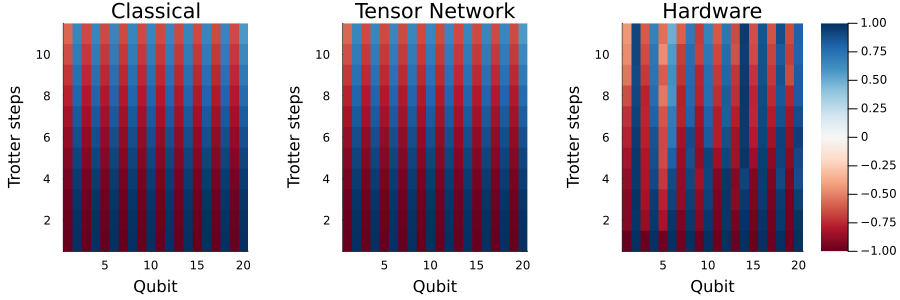
Dari sampel bitstring yang diperoleh dari hardware kuantum, kita hitung magnetisasi per site (nilai ekspektasi $\langle Z\rangle$ satu qubit) dengan merata-ratakan $(-1)^{b_i}$ atas semua shot, di mana $b_i$ adalah bit hasil ukur untuk qubit $i$ . Lalu kita plot magnetisasi sebagai heatmap terhadap qubit dan langkah Trotter, dengan membandingkan ketiga metode berdampingan: simulasi klasik eksak, simulasi tensor network tanpa noise, dan eksekusi di hardware.

# Compute expectation values
# 0 -> 1, 1 -> -1
z_expval(samples, i) = mean((-1)^s[i] for s in samples)

magnetizations = [z_expval(all_samples[i], q) for i in 1:length(all_samples), q in 1:N]

11×20 Matrix{Float64}:
 -0.996094  0.998047  -0.990234  0.998047  …  1.0       -0.988281  0.994141
 -0.925781  0.980469  -0.878906  0.96875      0.970703  -0.976562  0.988281
 -0.916016  0.992188  -0.837891  0.957031     0.962891  -0.966797  0.953125
 -0.884766  0.970703  -0.824219  0.90625      0.908203  -0.939453  0.892578
 -0.835938  0.96875   -0.814453  0.884766     0.931641  -0.902344  0.908203
 -0.777344  0.958984  -0.78125   0.871094  …  0.935547  -0.876953  0.939453
 -0.732422  0.933594  -0.767578  0.8125       0.884766  -0.835938  0.890625
 -0.650391  0.916016  -0.771484  0.771484     0.853516  -0.773438  0.837891
 -0.537109  0.902344  -0.705078  0.742188     0.875     -0.662109  0.833984
 -0.472656  0.923828  -0.652344  0.728516     0.839844  -0.695312  0.808594
 -0.4375    0.923828  -0.613281  0.681641  …  0.890625  -0.658203  0.8125

Ketiga panel di bawah menunjukkan magnetisasi site $\langle Z_i \rangle$ sebagai fungsi indeks qubit (sumbu x) dan langkah Trotter (sumbu y). Pada $\delta t = 0.05$ dengan $r_{\max} = 10$ , total waktu evolusi adalah $\tau = r_{\max} \cdot \delta t = 0.5$ , yang cukup singkat sehingga pola antiferomagnetik awal belum meluruh — ketiga metode menunjukkan pola yang berselang-seling dengan kuat. Hasil klasik dan tensor network sekarang sangat sesuai, yang menegaskan bahwa error Trotter kecil pada ukuran langkah ini. Hasil hardware secara umum mengikuti dua lainnya, meski beberapa qubit menyimpang dari simulasi lebih jauh daripada yang lain, mencerminkan variasi kualitas qubit di seluruh backend. Penyimpangan ini membesar pada langkah Trotter yang lebih akhir seiring kedalaman circuit bertambah.

# plot magnetization as a function of time
l = @layout [a{0.3w} b{0.3w} c{0.44w}]
plot(
    heatmap(classical_magnetizations, title="Classical", clims=(-1,1), color=:RdBu,
        xlabel="Qubit", ylabel="Trotter steps", colorbar=false),
    heatmap(tn_magnetizations, title="Tensor Network", clims=(-1,1), color=:RdBu,
        xlabel="Qubit", ylabel="Trotter steps", colorbar=false),
    heatmap(magnetizations, title="Hardware", clims=(-1,1), color=:RdBu,
        xlabel="Qubit", ylabel="Trotter steps", colorbar=true),
    layout=l, size=(900,300),
    bottom_margin=5mm, left_margin=5mm, right_margin=6mm
)

Output of the previous code cell

Contoh hardware skala besar

Langkah 1–4 dalam satu alur kerja

Sekarang kita gabungkan keempat langkah di atas menjadi satu alur kerja, pada skala di luar jangkauan simulasi klasik eksak. Alih-alih menguraikan magnetisasi site demi site, kita lacak satu ukuran skalar tunggal untuk keteraturan antiferomagnetik, yaitu magnetisasi staggered:

\langle M_s \rangle = \frac{1}{N} \sum_{i=1}^{N} (-1)^i \langle Z_i \rangle

Tanda yang berselang-seling dalam penjumlahan itu membuat sinyalnya terlihat. Untuk keadaan awal Néel $|0101\ldots01\rangle$ setiap suku menyumbang $+1$ , sehingga $\langle M_s\rangle = 1$ , sedangkan rata-rata biasa $\frac{1}{N}\sum_i \langle Z_i\rangle$ bernilai nol secara identik untuk semua $t$ . Saat medan transversal mengacak pola berselang-seling itu, $\langle M_s\rangle$ meluruh menuju $0$ , sehingga magnetisasi staggered memberi tahu kita seberapa banyak keteraturan awal yang bertahan selama evolusi waktu.

Kita juga memakai contoh ini untuk melihat bagaimana ukuran langkah Trotter memengaruhi akurasi. Kita tetapkan total waktu evolusi $T = 1.5$ dan variasikan jumlah langkah Trotter $r \in \{3, 6, 12\}$ , sehingga $\delta t = T/r$ . Di hardware, dua sumber error saling bersaing: $\delta t$ yang lebih kecil mengurangi error Trotter, tetapi memerlukan gate dua qubit yang proporsional lebih banyak, yang mengakumulasi lebih banyak noise hardware.

# -------------------------Step 1-------------------------
# Map classical inputs to a quantum problem.
N_large = 100
g_large = named_grid((N_large,))
h_large = fill(1.0, N_large)       # transverse field on every site
J_large = fill(1.0, N_large - 1)   # nearest-neighbor ZZ couplings on the chain

T_total = 1.5                    # fixed total evolution time
r_list = [3, 6, 12]       # varying Trotter steps; δt = T_total/r
sweep = [(r, k) for r in r_list for k in 0:r]

qc_list_large = [make_trotter_circuit(h_large, J_large, N_large, T_total/r, k)
                 for (r, k) in sweep]

# -------------------------Step 2-------------------------
# Optimize the problem for quantum hardware execution.
tqc_list_large = [transpile(qc, target)[1] for qc in qc_list_large]
# Print the 2q gate count and depth of the deepest circuit at each δt",
for r in r_list
    i = findfirst(==((r, r)), sweep)   # the k = r circuit reaches the full T_total
    println("  δt = $(round(T_total/r, digits=4))  →  $(r+1) time points, ",
        "deepest circuit = $(r) Trotter steps, ",
        "2q count = $(two_qubit_count(tqc_list_large[i])), ",
        "2q depth = $(two_qubit_depth(tqc_list_large[i]))")
end

# -------------------------Step 3-------------------------
# Execute using Qiskit primitives.
shots_large = 4096

job_list_large = [run_sampler_job(service, backend, tqc, shots_large)
                  for tqc in tqc_list_large]

δt = 0.5  →  4 time points, deepest circuit = 3 Trotter steps, 2q count = 594, 2q depth = 206
  δt = 0.25  →  7 time points, deepest circuit = 6 Trotter steps, 2q count = 1188, 2q depth = 218
  δt = 0.125  →  13 time points, deepest circuit = 12 Trotter steps, 2q count = 2376, 2q depth = 242

24-element Vector{QiskitIBMRuntime.Job}:
 QiskitIBMRuntime.Job(Ptr{QiskitIBMRuntime.LibQiskitIBMRuntime.Job} @0x0000000104c1a750)
 QiskitIBMRuntime.Job(Ptr{QiskitIBMRuntime.LibQiskitIBMRuntime.Job} @0x0000000102e0a270)
 QiskitIBMRuntime.Job(Ptr{QiskitIBMRuntime.LibQiskitIBMRuntime.Job} @0x0000000104c21a50)
 QiskitIBMRuntime.Job(Ptr{QiskitIBMRuntime.LibQiskitIBMRuntime.Job} @0x0000000102e05120)
 QiskitIBMRuntime.Job(Ptr{QiskitIBMRuntime.LibQiskitIBMRuntime.Job} @0x0000000104c2a6e0)
 QiskitIBMRuntime.Job(Ptr{QiskitIBMRuntime.LibQiskitIBMRuntime.Job} @0x0000000102e0d140)
 QiskitIBMRuntime.Job(Ptr{QiskitIBMRuntime.LibQiskitIBMRuntime.Job} @0x0000000102e0b640)
 QiskitIBMRuntime.Job(Ptr{QiskitIBMRuntime.LibQiskitIBMRuntime.Job} @0x0000000104c1a200)
 QiskitIBMRuntime.Job(Ptr{QiskitIBMRuntime.LibQiskitIBMRuntime.Job} @0x00000004b312eb90)
 QiskitIBMRuntime.Job(Ptr{QiskitIBMRuntime.LibQiskitIBMRuntime.Job} @0x0000000104c22060)
 QiskitIBMRuntime.Job(Ptr{QiskitIBMRuntime.LibQiskitIBMRuntime.Job} @0x00000004b31ea4e0)
 QiskitIBMRuntime.Job(Ptr{QiskitIBMRuntime.LibQiskitIBMRuntime.Job} @0x0000000104c1ccf0)
 QiskitIBMRuntime.Job(Ptr{QiskitIBMRuntime.LibQiskitIBMRuntime.Job} @0x0000000104c2af50)
 QiskitIBMRuntime.Job(Ptr{QiskitIBMRuntime.LibQiskitIBMRuntime.Job} @0x00000004b312ffb0)
 QiskitIBMRuntime.Job(Ptr{QiskitIBMRuntime.LibQiskitIBMRuntime.Job} @0x00000004b0e89700)
 QiskitIBMRuntime.Job(Ptr{QiskitIBMRuntime.LibQiskitIBMRuntime.Job} @0x0000000102e15070)
 QiskitIBMRuntime.Job(Ptr{QiskitIBMRuntime.LibQiskitIBMRuntime.Job} @0x0000000102e10d40)
 QiskitIBMRuntime.Job(Ptr{QiskitIBMRuntime.LibQiskitIBMRuntime.Job} @0x00000004af5a5d10)
 QiskitIBMRuntime.Job(Ptr{QiskitIBMRuntime.LibQiskitIBMRuntime.Job} @0x0000000102e12500)
 QiskitIBMRuntime.Job(Ptr{QiskitIBMRuntime.LibQiskitIBMRuntime.Job} @0x0000000102e14870)
 QiskitIBMRuntime.Job(Ptr{QiskitIBMRuntime.LibQiskitIBMRuntime.Job} @0x0000000102e10730)
 QiskitIBMRuntime.Job(Ptr{QiskitIBMRuntime.LibQiskitIBMRuntime.Job} @0x00000004b237ca60)
 QiskitIBMRuntime.Job(Ptr{QiskitIBMRuntime.LibQiskitIBMRuntime.Job} @0x00000004b2c713a0)
 QiskitIBMRuntime.Job(Ptr{QiskitIBMRuntime.LibQiskitIBMRuntime.Job} @0x0000000102e13e90)

# Run this cell to check the job status
# Run the following cell for post-processing after all jobs complete
for (i, job) in enumerate(job_list_large)
    r, k = sweep[i]
    println("Job $i (δt=$(round(T_total/r, digits=4)), k=$k): ",
            get_job_status(job, service))
end

Job 1 (δt=0.5, k=0): Completed
Job 2 (δt=0.5, k=1): Completed
Job 3 (δt=0.5, k=2): Completed
Job 4 (δt=0.5, k=3): Completed
Job 5 (δt=0.25, k=0): Completed
Job 6 (δt=0.25, k=1): Completed
Job 7 (δt=0.25, k=2): Completed
Job 8 (δt=0.25, k=3): Completed
Job 9 (δt=0.25, k=4): Completed
Job 10 (δt=0.25, k=5): Completed
Job 11 (δt=0.25, k=6): Completed
Job 12 (δt=0.125, k=0): Completed
Job 13 (δt=0.125, k=1): Completed
Job 14 (δt=0.125, k=2): Completed
Job 15 (δt=0.125, k=3): Completed
Job 16 (δt=0.125, k=4): Completed
Job 17 (δt=0.125, k=5): Completed
Job 18 (δt=0.125, k=6): Completed
Job 19 (δt=0.125, k=7): Completed
Job 20 (δt=0.125, k=8): Completed
Job 21 (δt=0.125, k=9): Completed
Job 22 (δt=0.125, k=10): Completed
Job 23 (δt=0.125, k=11): Completed
Job 24 (δt=0.125, k=12): Completed

# -------------------------Step 4-------------------------
# Post-process and return the result in the desired classical format.
# Run this cell after all jobs are completed

# ⟨M_s⟩ = (1/N) Σ (-1)^i ⟨Z_i⟩, averaged over hardware shots
function staggered_magnetization(samples::AbstractVector{<:AbstractVector}, n::Int)
    s = 0.0
    for sample in samples
        s += sum((-1)^i * (1 - 2 * sample[i]) for i in 1:n) / n
    end
    return s / length(samples)
end

all_samples_large = [get_sampler_job_results(job, service) for job in job_list_large]
mags_hardware = [staggered_magnetization(s, N_large) for s in all_samples_large]

24-element Vector{Float64}:
9880371093750097
697231445312484
44886718750000276
29333496093750067
9882324218750095
8109619140625324
6457958984374791
4808593749999992
36695312500000055
2963671875000012
23831542968750055
9884472656250093
8566455078125492
7951171875000282
7050732421874865
610673828124981
529980468749995
4656054687500018
4149316406250024
3799462890625011
35178710937500185
3185888671875003
31287597656250016
29621093750000077

Pada $N=100$ , solusi eksak dari solver ODE yang dipakai di atas tidak terjangkau, karena vektor keadaan saja akan membutuhkan $2^{100} \approx 10^{30}$ amplitudo. Sebagai gantinya, kita pakai simulasi tensor network tanpa noise untuk rantai 1D yang sama dengan langkah Trotter yang jauh lebih halus ( $r = 96$ , $\delta t \approx 0.016$ ) sebagai acuan, di mana error Trotter dapat diabaikan dibandingkan $\delta t$ mana pun yang kita jalankan di hardware. Acuan ini sendiri bersifat aproksimasi: error dominannya sekarang adalah pemotongan bond-dimension yang dibahas di atas, yang dilaporkan sebagai fidelitas pemotongan untuk setiap run.

apply_kwargs = (; maxdim=64, cutoff=1e-10, normalize_tensors=true)

# Calculate the staggered magnetization given a tensor network state
staggered_magnetization(ψ_bpc::BeliefPropagationCache, n::Int) =
    sum((-1)^q * m for (q, m) in enumerate(z_expvals_from_tn_state(ψ_bpc, n))) / n

# Evolve a TN state and record the staggered magnetization at each step.
function compute_staggered_magnetization_tn(δt::Real, nsteps::Int; record_every::Int = 1)
    init_gates = neel_state_gates(N_large)
    step_gates = trotter_step_gates(h_large, J_large, N_large, δt)

    ψ_bpc, fid = apply_gates_to_tn_state(init_gates, tn_initial_state(g_large); apply_kwargs)
    times = [0.0]
    mags = [staggered_magnetization(ψ_bpc, N_large)]
    for k in 1:nsteps
        ψ_bpc, fid_step = apply_gates_to_tn_state(step_gates, ψ_bpc; apply_kwargs)
        fid *= fid_step
        if k % record_every == 0
            push!(times, k * δt)
            push!(mags, staggered_magnetization(ψ_bpc, N_large))
        end
    end
    println("  δt=$(round(δt, digits=5)), $(nsteps) steps: truncation fidelity ≈ $(round(fid, digits=5))")
    (times, mags)
end

# If the fidelity drifts from 1, raise `maxdim` in `apply_kwargs`.
# Under current setting, the tensor network simulation takes ~ 3 minutes on a laptop.
println("Tensor-network reference:")
r_ref = 96
times_ref, mags_ref = compute_staggered_magnetization_tn(T_total / r_ref, r_ref; record_every = r_ref ÷ 12)

Tensor-network reference:
  δt=0.01562, 96 steps: truncation fidelity ≈ 1.0

([0.0, 0.125, 0.25, 0.375, 0.5, 0.625, 0.75, 0.875, 1.0, 1.125, 1.25, 1.375, 1.5], Float32[1.0, 0.9695576, 0.8870231, 0.77430177, 0.6560442, 0.5499543, 0.46285573, 0.39298016, 0.33518773, 0.28527063, 0.24147007, 0.20369667, 0.17206171])

Plot di bawah menunjukkan magnetisasi staggered terhadap waktu untuk ketiga ukuran langkah Trotter, dibandingkan dengan acuan tensor network tanpa noise (hitam putus-putus).

plt = plot(xlabel = "Time", ylabel = "Staggered magnetization",
    title = "N = $(N_large) on $(backend.name), T = $(T_total)",
    legend = :topright, ylims = (-0.05, 1.05), size = (820, 480),
    bottom_margin = 5mm, left_margin = 5mm)

# Plot tensor network reference
plot!(plt, times_ref, mags_ref, lw = 2, ls = :dash, color = :black,
      label = "tensor network, δt → 0")

# Plot hardware result per Trotter step size
for (r, stop) in zip(r_list, cumsum(r_list .+ 1))
    plot!(plt, range(0, T_total, length = r + 1), mags_hardware[(stop - r):stop],
          marker = :circle, markersize = 4, lw = 2,
          label = "hardware, δt = $(round(T_total / r, digits = 4))")
end
plt

Output of the previous code cell

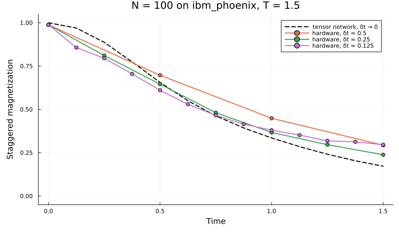
Secara keseluruhan, langkah Trotter terkasar $\delta t = 0.5$ (titik oranye) menunjukkan penyimpangan terbesar dari acuan tensor network, kemungkinan dengan kontribusi besar dari error Trotter. Pada langkah yang lebih halus $\delta t = 0.25$ (titik hijau), hasil hardware lebih sesuai dengan acuan. Pada langkah terhalus $\delta t = 0.125$ (titik ungu), error Trotter paling kecil, tetapi kesesuaiannya lebih buruk daripada pada $\delta t = 0.25$ . Dengan ukuran langkah separuhnya, setiap titik waktu memerlukan gate dua qubit dua kali lebih banyak, dan noise tambahan itu melebihi pengurangan error Trotter. Jadi memilih $\delta t$ untuk circuit Trotterisasi di hardware merupakan trade-off antara error Trotter dan noise yang terakumulasi dari gate tambahan.

Langkah berikutnya

Materi berikut mungkin menarik buat kamu:

Hasil pembelajaran​

Prasyarat​

Latar belakang​

Persyaratan​

Penyiapan​

Contoh simulator skala kecil​

Solusi eksak​

Simulasi skala kecil untuk circuit yang di-Trotterisasi​

Langkah 1: Petakan input klasik ke masalah kuantum​

Langkah 2: Optimalkan masalah untuk eksekusi di hardware kuantum​

Langkah 3: Eksekusi memakai primitif Qiskit​

Langkah 4: Pasca-proses dan kembalikan hasil dalam format klasik yang diinginkan​

Contoh hardware skala besar​

Langkah 1–4 dalam satu alur kerja​

Langkah berikutnya​