Munculnya ergodisitas di berbagai skala
Notebook ini membahas cara menjalankan dan menganalisis eksperimen di Onset of Ergodicity Across Scales on a Digital Quantum Processor [arXiv:2603.12236]: dari model ke circuit, dari bitstring ke entropi, dari data berderau ke hasil yang sudah dimitigasi, dan dari simulasi 16-qubit ke run 64-qubit di prosesor IBM Quantum® Nighthawk. Semua kodenya ada di sini, dan setiap fungsi didefinisikan di tempat pertama kali dibutuhkan.
| Waktu | Bagian |
|---|---|
| 0–1 menit | Persiapan |
| 1–6 menit | 1. Dari model ke circuit |
| 6–12 menit | 2. Apa yang diukur dan cara mengestimasinya |
| 12–19 menit | 3. Noise, dan cara membatalkannya |
| 19–24 menit | 4. Jalankan dalam skala besar |
| 24–33 menit | 5. Data hardware |
| 33–35 menit | Penutup |
Cara mengikutinya. Jalankan cell dari atas ke bawah. Kamu tidak perlu akun IBM Quantum; cell yang mengirim job hardware dimatikan, dan bagian 5 menganalisis run hardware yang tersimpan, yang diunduh oleh cell persiapan ke data/. Pertanyaan untuk diskusi ditandai Question; coba jawab dulu sebelum membuka jawabannya.
Persiapan
Membutuhkan Python 3.12 atau lebih baru dan paket-paket berikut:
-
Qiskit SDK v2.5 atau lebih baru, dengan dukungan visualisasi
-
Qiskit Runtime v0.49 atau lebih baru (
pip install qiskit-ibm-runtime) -
Qiskit Aer v0.17 atau lebih baru (
pip install qiskit-aer) -
Samplomatic v0.21 atau lebih baru (
pip install samplomatic) -
NumPy dan Matplotlib
Cell persiapan juga mengunduh run hardware yang tersimpan dan referensi MPS (sekitar 9 MB) ke data/, kecuali sudah ada di sana.
# Added by doQumentation — installs the packages this notebook needs if they are missing
import importlib.util

_needed = {"matplotlib": "matplotlib", "numpy": "numpy", "qiskit": "qiskit", "qiskit_aer": "qiskit-aer", "qiskit_ibm_runtime": "qiskit-ibm-runtime", "samplomatic": "samplomatic"}
_missing = [pip for module, pip in _needed.items()
            if importlib.util.find_spec(module) is None]
# One at a time, so a package that fails to install does not block the others
for _pip in _missing:
    %pip install -q {_pip}
if not _missing:
    print("\u2713 All required packages are installed")
from math import comb
from pathlib import Path
from urllib.request import urlretrieve

import matplotlib.pyplot as plt
import numpy as np
from qiskit import ClassicalRegister, QuantumCircuit, QuantumRegister
from qiskit.primitives import StatevectorSampler
from qiskit.quantum_info import (
    PauliLindbladMap,
    QubitSparsePauli,
    Statevector,
)
from qiskit.transpiler import generate_preset_pass_manager
from qiskit_aer import AerSimulator
from qiskit_aer.noise import NoiseModel, ReadoutError, depolarizing_error
from qiskit_aer.primitives import SamplerV2 as AerSampler

RUN_ON_HARDWARE = (
    False  # True submits the 8x8 jobs in section 4 (needs Nighthawk access)
)
COMPUTE_MPS_REFERENCES = False  # True recomputes the MPS references in section 5 (about 18 minutes)

# Download the saved hardware run and MPS references, unless they are already in data/
data_url = "https://raw.githubusercontent.com/Qiskit/documentation/main/datasets/tutorials/onset-of-ergodicity"
Path("data").mkdir(exist_ok=True)
for name in ("hardware_run.npz", "mps_references_all.npz"):
    if not Path("data", name).exists():
        urlretrieve(f"{data_url}/{name}", Path("data", name))
1. Dari model ke circuit
Gate dua-qubit
Setiap ikatan pada lattice mendapat gate dua-qubit yang sama, yang terdiri dari entangler Heisenberg diikuti medan acak:
dengan ditarik secara seragam dari untuk setiap gate.
Question. Bagaimana kamu mendekomposisi menjadi gate yang bisa dijalankan hardware?
Jawaban
Medannya mudah. adalah rotasi satu-qubit pada setiap qubit.
Entangler-nya bagian yang sulit. , dan saling komut, jadi bisa difaktorkan menjadi tiga rotasi, , dan . Masing-masing butuh dua CNOT, sehingga totalnya enam CNOT per gate.
Ada cara yang lebih baik. Gate dua-qubit apa pun bisa dibangun dari paling banyak tiga CNOT dan rotasi satu-qubit. Circuit optimalnya dimulai dari bentuk , dan entangler ini sudah punya bentuk itu dengan . Jadi ia langsung dipetakan ke tiga CNOT, dan sudut satu-qubit-nya linear terhadap . Kode eksperimen membangun gate dengan cara ini.
Di hardware, setiap gate dua-qubit menambah noise, jadi menghemat separuh jumlah CNOT itu penting.
def xxyyzz_gate(circuit, coupling, i, j):
    # exp(iJ(XX + YY + ZZ)) with three CNOTs; only the rotation angles depend on J
    circuit.rz(-np.pi / 2, j)
    circuit.cx(j, i)
    circuit.rz(np.pi / 2 - 2 * coupling, i)
    circuit.ry(2 * coupling - np.pi / 2, j)
    circuit.cx(i, j)
    circuit.ry(np.pi / 2 - 2 * coupling, j)
    circuit.cx(j, i)
    circuit.rz(np.pi / 2, i)

def heisenberg_gate(circuit, coupling, i, j, h_i, h_j):
    # The entangler first, then the random fields exp(i h Z)
    xxyyzz_gate(circuit, coupling, i, j)
    circuit.rz(-2 * h_i, i)
    circuit.rz(-2 * h_j, j)

h_i, h_j = 0.3, -0.7
gate = QuantumCircuit(2)
heisenberg_gate(gate, 0.05 * np.pi, 0, 1, h_i, h_j)
gate.draw("mpl")

Brickwork dan siklus Floquet
Gate-gate menutupi lattice persegi dalam empat sublayer ikatan yang tidak tumpang tindih, sebuah brickwork: ikatan horizontal mulai dari kolom genap, lalu kolom ganjil, lalu ikatan vertikal mulai dari baris genap, lalu baris ganjil. Qubit berada di situs .
def brickwork_layers(num_cols, num_rows):
    # Bonds of the square lattice, in the four sublayers of the brickwork
    def qubit(x, y):
        return y * num_cols + x

    layers = []
    for p in (0, 1):  # horizontal bonds starting on even, then odd, columns
        layers.append(
            [
                (qubit(x, y), qubit(x + 1, y))
                for y in range(num_rows)
                for x in range(p, num_cols - 1, 2)
            ]
        )
    for p in (0, 1):  # vertical bonds starting on even, then odd, rows
        layers.append(
            [
                (qubit(x, y), qubit(x, y + 1))
                for y in range(p, num_rows - 1, 2)
                for x in range(num_cols)
            ]
        )
    return layers

brickwork_layers(4, 4)
[[(0, 1), (2, 3), (4, 5), (6, 7), (8, 9), (10, 11), (12, 13), (14, 15)],
 [(1, 2), (5, 6), (9, 10), (13, 14)],
 [(0, 4), (1, 5), (2, 6), (3, 7), (8, 12), (9, 13), (10, 14), (11, 15)],
 [(4, 8), (5, 9), (6, 10), (7, 11)]]
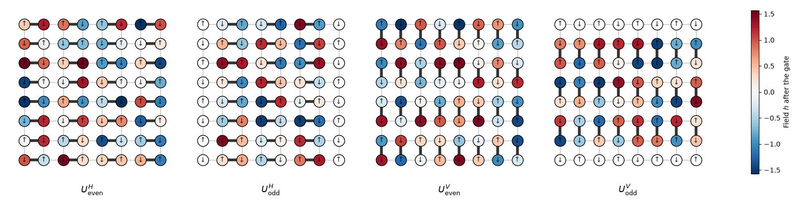
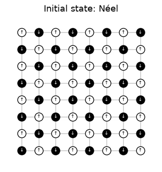
Keempat sublayer membentuk satu siklus Floquet. Siklus ini berulang kali dengan medan yang sama, jadi dinamikanya acak dalam ruang dan periodik dalam waktu. Circuit dimulai dari state Néel, dan adalah setengah panjang sisi lattice. Cell berikut menggambar satu siklus Floquet dari lattice hardware , sublayer demi sublayer, dengan medan dari run hardware, dalam gaya Gambar 5 di makalah. Ikatan tebal adalah gate dari setiap sublayer. Setiap qubit yang dikenai gate diwarnai sesuai medan acak yang kemudian diterimanya, dan qubit yang menganggur berwarna putih. Panah menunjukkan state awal Néel, dengan untuk . Gambar di makalah menerapkan sublayer vertikal lebih dulu; urutan mana pun tidak diperkirakan mengubah fisikanya.
# circuit structure, 8x8 system:
side = 8
all_bonds = [bond for layer in brickwork_layers(side, side) for bond in layer]

# get the disorder parameters for a given system:
def sample_disorder(num_cols, num_rows, rng):
    # One pair of fields (h_i, h_j) per gate, reused in every Floquet cycle
    return [
        [
            (bond, tuple(rng.uniform(-np.pi / 2, np.pi / 2, 2)))
            for bond in layer
        ]
        for layer in brickwork_layers(num_cols, num_rows)
    ]

# build the structure for the 8x8 system
example_disorder = sample_disorder(
    side, side, np.random.default_rng(7)
)  # the hardware fields (section 4)
titles = [
    r"$U^H_\mathrm{even}$",
    r"$U^H_\mathrm{odd}$",
    r"$U^V_\mathrm{even}$",
    r"$U^V_\mathrm{odd}$",
]
norm = plt.Normalize(-np.pi / 2, np.pi / 2)
cmap = plt.get_cmap("RdBu_r")

fig, axes = plt.subplots(1, 4, figsize=(16, 4.8), layout="constrained")
for ax, title, sublayer in zip(axes, titles, example_disorder):
    for i, j in all_bonds:
        ax.plot(
            [i % side, j % side],
            [i // side, j // side],
            color="0.75",
            lw=1,
            zorder=0,
        )
    fields = {}
    for (i, j), (h_i, h_j) in sublayer:
        ax.plot(
            [i % side, j % side],
            [i // side, j // side],
            color="0.2",
            lw=4,
            zorder=1,
        )
        fields[i], fields[j] = h_i, h_j
    for q in range(side * side):
        x, y = q % side, q // side
        ax.scatter(
            x,
            y,
            s=260,
            color=cmap(norm(fields[q])) if q in fields else "white",
            edgecolor="black",
            zorder=2,
        )
        ax.text(
            x,
            y,
            "↓" if (x + y) % 2 else "↑",
            ha="center",
            va="center",
            fontsize=9,
            zorder=3,
        )
    ax.set_aspect("equal")
    ax.set_xlim(-1, side)  # padding, so the panels read as separate steps
    ax.set_ylim(side, -1)
    ax.axis("off")
    ax.set_title(title, y=-0.1, fontsize=13)
fig.colorbar(
    plt.cm.ScalarMappable(norm=norm, cmap=cmap),
    ax=axes,
    shrink=0.7,
    label="Field $h$ after the gate",
)
plt.show()
Tentukan state awal.
# initial state
def neel_state(circuit, num_cols, num_rows, layout):
    for y in range(num_rows):
        for x in range(num_cols):
            if (x + y) % 2 == 1:
                circuit.x(layout[y * num_cols + x])
# The initial Néel state: |1⟩ (black, ↓) on odd sites, |0⟩ (white, ↑) on even sites

fig, ax = plt.subplots(figsize=(4, 4.4))
for i, j in all_bonds:
    ax.plot(
        [i % side, j % side],
        [i // side, j // side],
        color="0.75",
        lw=1,
        zorder=0,
    )
for q in range(side * side):
    x, y = q % side, q // side
    excited = (x + y) % 2 == 1
    ax.scatter(
        x,
        y,
        s=150,
        color="black" if excited else "white",
        edgecolor="black",
        zorder=2,
    )
    ax.text(
        x,
        y,
        "↓" if excited else "↑",
        ha="center",
        va="center",
        fontsize=7,
        color="white" if excited else "black",
        zorder=3,
    )
ax.set_aspect("equal")
ax.set_xlim(-1, side)
ax.set_ylim(side, -1)
ax.axis("off")
ax.set_title("Initial state: Néel", fontsize=13)
plt.show()
# actual circuit construction:
def heisenberg_floquet_circuit(
    num_cols, num_rows, coupling, num_cycles, disorder, measure=True
):
    num_qubits = num_cols * num_rows
    circuit = QuantumCircuit(num_qubits)
    neel_state(circuit, num_cols, num_rows, list(range(num_qubits)))
    cycle = QuantumCircuit(num_qubits)
    for sublayer in disorder:
        for (i, j), (h_i, h_j) in sublayer:
            heisenberg_gate(cycle, coupling, i, j, h_i, h_j)
    for _ in range(num_cycles):
        circuit.compose(cycle, inplace=True)
    if measure:
        circuit.measure_all()
    return circuit
Contoh
Simulasi memakai lattice dengan dua siklus, dan kopling yang dipelajari di makalah. Satu set medan dipakai ulang untuk setiap kopling.
# simulation parameters:
num_cols = num_rows = 4
num_qubits = num_cols * num_rows
num_cycles = 2
couplings = (
    np.array([0.005, 0.01, 0.02, 0.03, 0.04, 0.05, 0.06, 0.08, 0.10, 0.125])
    * np.pi
)
disorder = sample_disorder(num_cols, num_rows, np.random.default_rng(42))

# circuit construction:
logical_circuits = [
    heisenberg_floquet_circuit(
        num_cols, num_rows, coupling, num_cycles, disorder
    )
    for coupling in couplings
]
logical_circuits[5].draw(output="mpl", fold=-1)

# transpiling the circuit:
pass_manager = generate_preset_pass_manager(
    optimization_level=3,
    basis_gates=["cz", "rz", "sx", "x"],
    seed_transpiler=7,
)
circuits = [pass_manager.run(circuit) for circuit in logical_circuits]

def two_qubit_stats(circuit):
    count = sum(1 for inst in circuit.data if inst.operation.num_qubits == 2)
    depth = circuit.depth(lambda inst: inst.operation.num_qubits == 2)
    return count, depth

stats = {two_qubit_stats(circuit) for circuit in circuits}
assert len(stats) == 1, "the CZ structure should not depend on J"
num_cz, depth = stats.pop()
print(
    f"{num_qubits} qubits: {num_cz} CZ gates in {depth} layers, for every coupling"
)
circuits[5].draw("mpl", fold=-1, scale=0.4)
16 qubits: 144 CZ gates in 24 layers, for every coupling

Compiler yang canggih tidak diperlukan, karena circuit (dan eksperimen) dirancang untuk IBM Nighthawk.
Simulasikan lattice
Untuk lattice , kamu bisa melakukan keduanya: menghitung state eksak di setiap kopling, dan men-sample setiap circuit dengan 10.000 shot, seperti yang dilakukan eksperimen. Shot disimpan dengan bentuk (batch, shot, qubit), tata letak yang sama dengan randomisasi di data hardware. Di sini semua 10.000 shot membentuk satu batch, jadi bootstrap atas batch tidak menambah shot noise, dan error bar di plot berikut hanya menunjukkan sebaran antar posisi marginal.
exact_states = [
    Statevector(
        heisenberg_floquet_circuit(
            num_cols, num_rows, c, num_cycles, disorder, measure=False
        )
    )
    for c in couplings
]

shots = 10_000
results = (
    StatevectorSampler(default_shots=shots, seed=1234).run(circuits).result()
)

# the output of the simulation for the 10 couplings
bits = [
    result.data.meas.to_bool_array(order="little").reshape(
        1, 10_000, num_qubits
    )
    for result in results
]

print(bits[0])
[[[False  True False ... False  True False]
  [False  True False ... False  True False]
  [False  True False ... False  True False]
  ...
  [False  True False ... False  True False]
  [False  True False ... False  True False]
  [False  True False ... False  True False]]]
2. Apa yang diukur dan cara mengestimasinya
IPR dan collision entropy
Untuk marginal dengan qubit dan distribusi bitstring , besaran yang diestimasi adalah inverse participation ratio (IPR) dari distribusi marginal, dan dari situ collision entropy:
juga merupakan probabilitas bahwa dua shot sama pada marginal tersebut. State produk punya , dan state acak punya , jadi naik dari 0 sampai sekitar bit saat marginal menjadi acak.
Estimator 1: hitung pasangan shot
Question. Bagaimana kamu mengestimasi besaran ini dari shot-mu?
Jawaban
Estimator naif menghitung setiap dari shot sebagai , lalu menjumlahkan . Estimator ini bias.
menghitung setiap shot sebagai sama dengan dirinya sendiri, yang mendorong estimasi naik: rata-rata hasilnya dan bukan . Karena adalah probabilitas bahwa dua shot sama, hitung hanya pasangan shot yang berbeda:
Ini tidak bias, dan inilah yang dihitung ipr_from_shots di bawah.
# IPR expectation values:

# refactor this function cause it does not scale
def ipr_from_shots(bits):
    # Pair-counting estimate of the IPR of a marginal: the fraction of pairs of different shots
    # that agree on it. bits holds the marginal's qubits only, with shape (randomizations, shots,
    # qubits), and all randomizations are pooled.
    n = bits.shape[-1]
    outcomes = bits @ 2 ** np.arange(
        n
    )  # each shot's marginal bitstring, read as an integer
    counts = np.bincount(outcomes.ravel())  # how often each outcome occurs
    total = counts.sum()
    return float((counts * (counts - 1)).sum() / (total * (total - 1)))

def collision_entropy(ipr):
    return -np.log2(ipr)
Estimator 2: ekspansi Parseval
IPR juga bisa ditulis lewat paritas dari semua subhimpunan tak kosong dari marginal:
Bentuk ini penting karena metode error mitigation seperti PEA bekerja pada nilai ekspektasi, bukan pada probabilitas. Satu qubit: Probabilitas hasilnya adalah dan , jadi
Marginal : Dengan qubit-nya diberi label , marginal punya paritas: 4 qubit tunggal, 6 pasangan, 4 triplet, dan seluruh marginal, jadi
def parity_supports(patch):
    # All nonempty subsets S of the marginal
    return sorted(
        [
            tuple(q for k, q in enumerate(patch) if mask & (1 << k))
            for mask in range(1, 1 << len(patch))
        ],
        key=len,
    )

def parity_expectation_values(bits, supports):
    # Shot-averaged <Z_S> for every support, per randomization
    signs = 1 - 2 * bits.astype(np.int8)
    return np.stack(
        [signs[..., list(s)].prod(axis=-1).mean(axis=-1) for s in supports],
        axis=-1,
    )

# Example: the parities of a 3-qubit marginal made of lattice qubits 5, 6, and 9
print(parity_supports([5, 6, 9]))
print(f"A 3×3 marginal has {len(parity_supports(range(9)))} parities")
[(5,), (6,), (9,), (5, 6), (5, 9), (6, 9), (5, 6, 9)]
A 3×3 marginal has 511 parities
Rata-rata atas marginal
Fungsi tambahan yang berguna: nilai Haar, memilih marginal, bootstrapping, dan averaging.
# functions for the Haar values on plots:
def haar_ipr(num_patch, num_qubits):
    # Mean IPR of a marginal for Haar-random states in the sector with num_qubits // 2 ones
    weight = num_qubits // 2
    dimension = comb(num_qubits, weight)
    total = 0
    for k in range(num_patch + 1):  # k ones on the marginal
        rest = (
            comb(num_qubits - num_patch, weight - k) if weight - k >= 0 else 0
        )
        total += comb(num_patch, k) * rest * (rest + 1)
    return total / (dimension * (dimension + 1))

def haar_entropy(num_patch, num_qubits):
    return collision_entropy(haar_ipr(num_patch, num_qubits))

# definitions of positions in the lattice:
def patch_qubits(anchor, shape, num_cols):
    # Lattice indices of a rectangular marginal with its top-left corner at anchor
    (x0, y0), (width, height) = anchor, shape
    return [
        (y0 + dy) * num_cols + (x0 + dx)
        for dy in range(height)
        for dx in range(width)
    ]

def all_positions(shape, num_cols, num_rows):
    # Every placement of a (width, height) marginal on the lattice
    width, height = shape
    return [
        patch_qubits((x, y), shape, num_cols)
        for y in range(num_rows - height + 1)
        for x in range(num_cols - width + 1)
    ]

# bootstrapping for error bars:
bootstrap_rng = np.random.default_rng(0)

def bootstrap_error(statistic, *samples, axis=0, num_resamples=50):
    # Shot noise of a statistic, from resampling the randomizations (along axis of every
    # sample) with replacement
    values = []
    for _ in range(num_resamples):
        resampled = [
            np.take(
                x,
                bootstrap_rng.integers(0, x.shape[axis], x.shape[axis]),
                axis=axis,
            )
            for x in samples
        ]
        values.append(statistic(*resampled))
    return float(np.std(values, ddof=1))

# averaging the ipr over marginals:
def average_ipr(iprs, shot_errors):
    # iprs and shot_errors have shape (positions, couplings). The mean IPR over positions, and its
    # error: the spread between positions plus the shot noise of each (law of total variance)
    iprs, shot_errors = np.asarray(iprs), np.asarray(shot_errors)
    count = len(iprs)
    variance = (
        iprs.var(axis=0, ddof=1) / count
        + (shot_errors**2).sum(axis=0) / count**2
    )
    return iprs.mean(axis=0), np.sqrt(variance)
# Calculating exact simulation entropies:
patch_shapes = {
    "1×1": (1, 1),
    "1×2": (2, 1),
    "2×2": (2, 2),
    "2×3": (3, 2),
    "3×3": (3, 3),
}

# calculate the exact entropies:
sim_positions = {
    label: all_positions(shape, num_cols, num_rows)
    for label, shape in patch_shapes.items()
}
exact_iprs = {  # shape (positions, couplings)
    label: np.array(
        [
            [(s.probabilities(qargs=q) ** 2).sum() for s in exact_states]
            for q in qubit_lists
        ]
    )
    for label, qubit_lists in sim_positions.items()
}
exact_entropies = {
    label: collision_entropy(v.mean(axis=0))
    for label, v in exact_iprs.items()
}

# Average IPR of every shape over its positions, from the sampled shots, then the entropy
iprs_from_shots = {}  # per shape: average IPR and its error, at every coupling
entropies_from_shots = {}  # per shape: average entropy and its error, at every coupling
for label, qubit_lists in sim_positions.items():
    iprs = [[ipr_from_shots(b[:, :, q]) for b in bits] for q in qubit_lists]

    # bootstrapping over subsampling for error bars:
    errors = [
        [bootstrap_error(ipr_from_shots, b[:, :, q]) for b in bits]
        for q in qubit_lists
    ]
    ipr, ipr_error = average_ipr(iprs, errors)
    iprs_from_shots[label] = (ipr, ipr_error)
    entropies_from_shots[label] = (
        collision_entropy(ipr),
        ipr_error / (ipr * np.log(2)),
    )
# Now plot the average IPR on the left, and the same averages as entropies on the right
colors = plt.cm.plasma(np.linspace(0.05, 0.8, len(patch_shapes)))
fig, (ax_ipr, ax_entropy) = plt.subplots(1, 2, figsize=(12.8, 4.2))
for (label, qubit_lists), color in zip(sim_positions.items(), colors):
    n = len(qubit_lists[0])
    ipr, ipr_error = iprs_from_shots[label]
    entropy, entropy_error = entropies_from_shots[label]
    # Left: the average IPR, with its exact value and its random-state value
    ax_ipr.axhline(haar_ipr(n, num_qubits), color=color, ls="dashdot", lw=0.9)
    ax_ipr.plot(
        couplings / np.pi, exact_iprs[label].mean(axis=0), color=color
    )
    ax_ipr.errorbar(
        couplings / np.pi,
        ipr,
        yerr=ipr_error,
        fmt="o",
        color=color,
        mec="white",
        ms=7,
        capsize=3,
        label=f"{label} ({len(qubit_lists)} positions)",
    )
    # Right: the average collision entropy
    ax_entropy.axhline(
        haar_entropy(n, num_qubits), color=color, ls="dashdot", lw=0.9
    )
    ax_entropy.plot(couplings / np.pi, exact_entropies[label], color=color)
    ax_entropy.errorbar(
        couplings / np.pi,
        entropy,
        yerr=entropy_error,
        fmt="o",
        color=color,
        mec="white",
        ms=7,
        capsize=3,
        label=f"{label} ({len(qubit_lists)} positions)",
    )
ax_ipr.set_yscale("log")
ax_ipr.set_ylabel("Average IPR")
ax_entropy.set_ylabel("Average collision entropy (bits)")
for ax in (ax_ipr, ax_entropy):
    ax.set_xlabel("Coupling $J/\\pi$")
fig.suptitle("Exact (lines) and sampled (dots), 4×4 lattice, 2 cycles")
ax_entropy.legend(title="Marginal", loc="upper left")
fig.tight_layout()
plt.show()
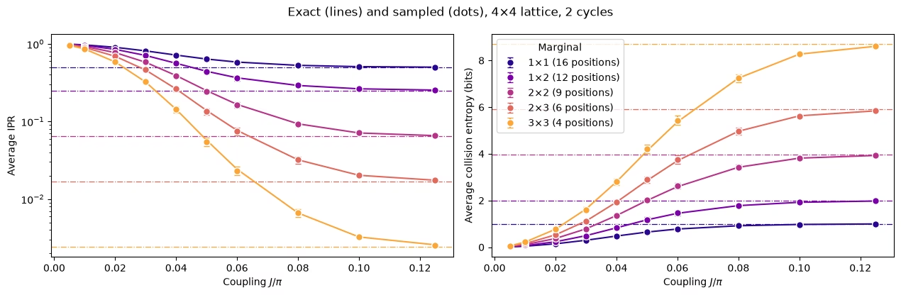
Setiap bentuk marginal naik dengan mulus menuju nilai state acaknya, dan marginal yang lebih besar mencapainya pada yang lebih besar.
3. Noise, dan cara menghilangkannya
Simulasi dengan noise
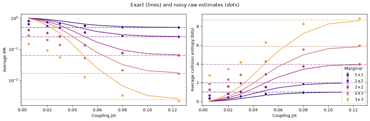
Sekarang tambahkan noise: noise depolarizing dua-qubit 1% pada setiap gate CZ dan error readout 3% pada setiap qubit, disampel dengan Sampler Qiskit Aer. Dengan 144 gate CZ di circuit, noise ini jauh lebih kecil daripada yang dialami circuit hardware 8×8, tetapi cukup untuk melihat efeknya. Simulasi memakai enam coupling dan masing-masing 4.000 shot, dan butuh sekitar 1,5 menit.
Pertanyaan. Sebelum kamu menjalankannya: apakah noise membuat sistem terlihat lebih terthermalisasi atau kurang terthermalisasi?
Jawaban
Lebih. Noise mengacak hasil, sehingga setiap distribusi marginal terdorong ke arah seragam, jadi IPR mentah turun dan entropi naik. Tanpa mitigasi, noise terlihat seperti thermalisasi yang sebenarnya tidak ada, dan crossover muncul terlalu awal.
# define the noise model

noise_model = NoiseModel()
# two qubit depolarizing noise:
noise_model.add_all_qubit_quantum_error(depolarizing_error(0.01, 2), ["cz"])
# symmetric readout noise:
noise_model.add_all_qubit_readout_error(
    ReadoutError([[0.97, 0.03], [0.03, 0.97]])
)

# simulation is done using trajectories
noisy_sampler = AerSampler(
    default_shots=4000,
    seed=1,
    options={"backend_options": {"noise_model": noise_model}},
)

# choose a subset of J values for speed:
noisy_indices = [
    0,
    2,
    3,
    5,
    7,
    9,
]  # J/π = 0.005, 0.02, 0.03, 0.05, 0.08, 0.125
noisy_results = noisy_sampler.run(
    [circuits[k] for k in noisy_indices]
).result()

# No twirling here, so the 20 "randomizations" are just batches of 200 shots
noisy_bits = {
    k: result.data.meas.to_bool_array(order="little").reshape(
        20, 200, num_qubits
    )
    for k, result in zip(noisy_indices, noisy_results)
}
# Calculating noisy entropies

# Average IPR of every shape over its positions, from the noisy shots, then the entropy
noisy_iprs = {}  # per shape: average IPR and its error, at every noisy coupling
noisy_entropies = {}  # per shape: average entropy and its error, at every noisy coupling
for label, qubit_lists in sim_positions.items():
    iprs = [
        [ipr_from_shots(noisy_bits[k][:, :, q]) for k in noisy_indices]
        for q in qubit_lists
    ]

    # bootstrapping over subsampling for error bars:
    errors = [
        [
            bootstrap_error(ipr_from_shots, noisy_bits[k][:, :, q])
            for k in noisy_indices
        ]
        for q in qubit_lists
    ]
    ipr, ipr_error = average_ipr(iprs, errors)
    noisy_iprs[label] = (ipr, ipr_error)
    noisy_entropies[label] = (
        collision_entropy(ipr),
        ipr_error / (ipr * np.log(2)),
    )
fig, (ax_ipr, ax_entropy) = plt.subplots(1, 2, figsize=(12.8, 4.2))
for (label, qubit_lists), color in zip(sim_positions.items(), colors):
    n = len(qubit_lists[0])
    ipr, ipr_error = noisy_iprs[label]
    entropy, entropy_error = noisy_entropies[label]
    # Left: the average IPR, with its exact value and its random-state value
    ax_ipr.axhline(haar_ipr(n, num_qubits), color=color, ls="dashdot", lw=0.9)
    ax_ipr.plot(
        couplings / np.pi, exact_iprs[label].mean(axis=0), color=color
    )
    ax_ipr.errorbar(
        couplings[noisy_indices] / np.pi,
        ipr,
        yerr=ipr_error,
        fmt="o",
        color=color,
        mec="white",
        ms=7,
        capsize=3,
        label=label,
    )
    # Right: the same averages as entropies
    ax_entropy.axhline(
        haar_entropy(n, num_qubits), color=color, ls="dashdot", lw=0.9
    )
    ax_entropy.plot(couplings / np.pi, exact_entropies[label], color=color)
    ax_entropy.errorbar(
        couplings[noisy_indices] / np.pi,
        entropy,
        yerr=entropy_error,
        fmt="o",
        color=color,
        mec="white",
        ms=7,
        capsize=3,
        label=label,
    )
ax_ipr.set_yscale("log")
ax_ipr.set_ylabel("Average IPR")
ax_entropy.set_ylabel("Average collision entropy (bits)")
for ax in (ax_ipr, ax_entropy):
    ax.set_xlabel("Coupling $J/\\pi$")
fig.suptitle("Exact (lines) and noisy raw estimates (dots)")
ax_entropy.legend(title="Marginal", loc="lower right")
fig.tight_layout()
plt.show()
Brainstorm: bagaimana cara menghilangkannya?
Pendekatan yang disarankan
Pada kecil, state hampir tidak terentangle, jadi jawaban idealnya murah dihitung secara klasik, bahkan untuk 64 qubit. Ini menyarankan kita mengukur efek noise pada coupling kalibrasi kecil dan mengoreksi semua coupling lain dengannya. Ada dua cara yang wajar untuk melakukannya, disebut low-entanglement calibration (LEC):
LEC pada IPR. Skalakan kelebihan IPR di atas nilainya untuk distribusi seragam, , dengan satu faktor per marginal:
LEC pada nilai ekspektasi . Skalakan setiap paritas dari marginal dengan faktornya sendiri, lalu bangun kembali IPR dengan rumus Parseval:
Dalam kode, setiap paritas terskala yang dikuadratkan di-debias dengan mengurangi variansnya, seperti di bagian 2.
Keduanya sama jika setiap sama dengan .
Question. What are the pros and cons of these methods?
Jawaban
Pros
-
Murah: tidak butuh data tambahan dari device, hanya simulasi klasik pada .
-
Memakai struktur circuit: kedalaman circuit dan layer CZ tidak berubah terhadap , jadi noise pada sama dengan noise pada setiap lainnya.
Cons
- Mengasumsikan efek noise pada observable tidak bergantung pada : noisenya sendiri sama, tetapi cara noise meredam IPR atau tiap bisa berubah saat membesar.
Kedua metode pada simulasi dengan noise
# function to mitigate the IPR signal:
def mitigate_ipr_w_lec(
    ipr_raw, ipr_raw_calibration, ipr_ideal_calibration, num_patch
):
    # LEC on the IPR: one factor R0 for the excess over the uniform value
    uniform = 2.0**-num_patch
    factor = (ipr_ideal_calibration - uniform) / (
        ipr_raw_calibration - uniform
    )
    return uniform + factor * (ipr_raw - uniform)

# function used to calculate the target <Z> expectation values
def parities_from_probabilities(probabilities):
    # Ideal <Z_S> from a marginal distribution, in parity_supports order: subsets
    # by size, and in bitmask order within each size
    outcomes = np.arange(len(probabilities))
    masks = np.array(sorted(range(1, len(probabilities)), key=int.bit_count))
    signs = (-1.0) ** np.bitwise_count(outcomes[:, None] & masks[None, :])
    return np.asarray(probabilities) @ signs

# calculate boosting factors:
def lec_z_factors(calibration_parities, ideal_parities):
    # LEC on <Z>: one factor r_S per parity, from data with shape (randomizations, supports).
    return ideal_parities / calibration_parities.mean(axis=0)

# function to mitigate the IPR from <Z> expectation values:
def mitigate_ipr_w_lec_on_parities(
    parities, calibration_parities, ideal_calibration_parities, num_patch
):
    # LEC on <Z>: rescale each parity by its factor r_S = ideal / raw at J0, then rebuild the IPR
    # with Parseval. parities and calibration_parities have shape (randomizations, supports).
    # Each squared, rescaled parity is debiased by subtracting its variance, which to first
    # order combines the shot noise at J. The shot noise of r_S from J0 is omitted; including it
    # does not change the results.
    factors = lec_z_factors(calibration_parities, ideal_calibration_parities)
    mean = parities.mean(axis=0)  # mean over the twirling instances
    variance = parities.var(axis=0, ddof=1) / len(
        parities
    )  # variance of the mean
    rescaled = factors * mean
    rescaled_variance = factors**2 * variance
    return float((1 + np.sum(rescaled**2 - rescaled_variance)) / 2**num_patch)
def lec_estimates(patch_bits, parities, ideal, calibration, num_patch):
    # LEC on the IPR and on <Z> for one marginal position, at every coupling: values and shot
    # noise. patch_bits (the bits of the marginal only) and parities are per coupling, with
    # randomizations first.
    q_ideal = (ideal**2).sum()
    ideal_parities = parities_from_probabilities(ideal)

    def ipr_statistic(b, c):
        return mitigate_ipr_w_lec(
            ipr_from_shots(b), ipr_from_shots(c), q_ideal, num_patch
        )

    def z_statistic(p, c):
        return mitigate_ipr_w_lec_on_parities(p, c, ideal_parities, num_patch)

    values = {"LEC on IPR": [], "LEC on ⟨Z⟩": []}
    errors = {"LEC on IPR": [], "LEC on ⟨Z⟩": []}
    for k in range(len(patch_bits)):
        if (
            k == calibration
        ):  # both match the ideal value at J0 by construction
            for method in values:
                values[method].append(q_ideal)
                errors[method].append(0.0)
            continue
        values["LEC on IPR"].append(
            ipr_statistic(patch_bits[k], patch_bits[calibration])
        )
        errors["LEC on IPR"].append(
            bootstrap_error(
                ipr_statistic, patch_bits[k], patch_bits[calibration]
            )
        )
        values["LEC on ⟨Z⟩"].append(
            z_statistic(parities[k], parities[calibration])
        )
        errors["LEC on ⟨Z⟩"].append(
            bootstrap_error(z_statistic, parities[k], parities[calibration])
        )
    return values, errors

# getting all the data:
calibration_index = 0  # index of J0 = 0.005π in noisy_indices
mitigated = {
    "LEC on IPR": {},
    "LEC on ⟨Z⟩": {},
}  # per shape: (values, errors), each (positions, couplings)
for label, qubit_lists in sim_positions.items():
    n = len(qubit_lists[0])
    per_position = []
    for qubits in qubit_lists:
        supports = parity_supports(qubits)
        parities = [
            parity_expectation_values(noisy_bits[k], supports)
            for k in noisy_indices
        ]
        patch_bits = [noisy_bits[k][:, :, qubits] for k in noisy_indices]
        ideal = exact_states[noisy_indices[calibration_index]].probabilities(
            qargs=qubits
        )
        per_position.append(
            lec_estimates(patch_bits, parities, ideal, calibration_index, n)
        )
    for method in mitigated:
        mitigated[method][label] = (
            [p[0][method] for p in per_position],
            [p[1][method] for p in per_position],
        )

# Average over positions, then the entropy, for both methods
mitigated_entropies = {
    method: {} for method in mitigated
}  # per method and shape: entropy and its error
for method, by_shape in mitigated.items():
    for label, (values, errors) in by_shape.items():
        ipr, ipr_error = average_ipr(values, errors)
        mitigated_entropies[method][label] = (
            collision_entropy(ipr),
            ipr_error / (ipr * np.log(2)),
        )  # log here comes from error propagation
# Plot the data mitigated with both methods:

fig, axes = plt.subplots(1, 2, figsize=(12.8, 4.2), sharey=True)
for ax, (method, by_shape) in zip(axes, mitigated_entropies.items()):
    for (label, qubit_lists), color in zip(sim_positions.items(), colors):
        entropy, error = by_shape[label]
        ax.axhline(
            haar_entropy(len(qubit_lists[0]), num_qubits),
            color=color,
            ls="dashdot",
            lw=0.9,
        )
        ax.plot(couplings / np.pi, exact_entropies[label], color=color)
        ax.errorbar(
            couplings[noisy_indices] / np.pi,
            entropy,
            yerr=error,
            fmt="o",
            color=color,
            mec="white",
            ms=7,
            capsize=3,
            label=label,
        )
    ax.set_title(f"{method} (lines: exact)")
    ax.set_xlabel("Coupling $J/\\pi$")
axes[0].set_ylabel("Average collision entropy (bits)")
axes[0].legend(title="Marginal", loc="lower right")
fig.tight_layout()
plt.show()

# add the noisy data here too
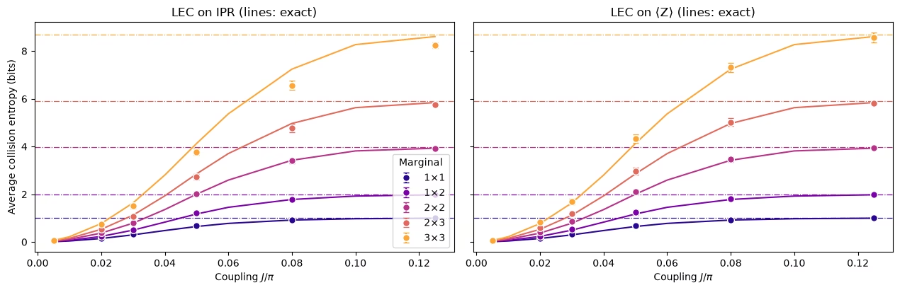
Kedua metode menghilangkan sebagian besar kerusakan: estimasi mentah di plot sebelumnya terlalu acak, dan estimasi yang sudah dimitigasi mengikuti kurva eksak. Perbedaannya terlihat pada marginal yang lebih besar.
Untuk marginal kecil, kedua metode berhasil. Untuk marginal , LEC pada jelas lebih dekat.
Mengapa LEC pada IPR menghasilkan entropi terlalu kecil. Entropi terlalu kecil berarti IPR terlalu besar: LEC pada IPR menggelembungkannya berlebihan. Metode ini mengasumsikan bahwa noise meredam kontribusi setiap ke IPR dengan faktor yang sama. Pada , setiap mendekati , jadi semua string berkontribusi sama, dan kebanyakan string punya bobot sedang: dari 511 string marginal , 252 punya bobot 4 atau 5, dan hanya sembilan yang berbobot 1. Noise meredam string makin kuat jika bobotnya makin tinggi (error readout saja meredam string berbobot- sebesar ), jadi faktor tunggal terutama ditentukan oleh peredaman string berbobot sedang. Saat membesar, berbobot lebih tinggi meluruh paling cepat, dan IPR makin banyak dibawa oleh string berbobot rendah, yang diredam noise lebih sedikit. Mengangkat string-string itu dengan faktor yang dipelajari terutama dari string yang lebih kuat teredam akan menggelembungkan IPR berlebihan. Efeknya tumbuh seiring ukuran marginal, karena marginal yang lebih besar punya rentang bobot lebih lebar. Efeknya terbesar pada menengah, setelah campuran string bergeser tetapi selagi kelebihan IPR di atas nilai serAGAMnya masih berarti.
Mengapa LEC pada salah ke arah sebaliknya. Metode ini menskalakan tiap string dengan faktornya sendiri, jadi pergeseran antar bobot tidak memengaruhinya. Ia hanya mengasumsikan bahwa tiap string mempertahankan peredamannya pada . Saat membesar, tiap menyebar ke operator berbobot lebih tinggi, yang menerima lebih banyak noise daripada pada , sehingga faktornya sedikit kurang mengoreksi dan entropi keluar sedikit terlalu tinggi.
Jadi prediksi yang perlu diuji di hardware adalah: makin besar marginal, makin besar kemungkinan LEC pada menang. Di hardware, noise lebih kuat dan tidak berbentuk yang dikenal.
4. Jalankan dalam skala besar
Eksperimen hardware menjalankan lattice dengan empat siklus: 64 qubit dan 1.344 gate CZ dalam 48 layer, pada sembilan coupling. Lima hal berubah dibandingkan simulasi:
-
Noise harus dipelajari, yang hanya berhasil jika layer CZ-nya tetap.
-
Twirling mengubah noise tiap layer menjadi channel Pauli, yang bisa dipelajari dan diamplifikasi.
-
Dynamical decoupling (DD) melindungi qubit yang menganggur.
-
Amplifikasi noise untuk PEA berjalan dalam job yang sama dengan data utama.
-
Simulasi MPS pada kecil menyediakan referensi klasik untuk mitigasi error berbasis LEC.
Cell yang butuh backend hanya berjalan saat RUN_ON_HARDWARE bernilai True. Simulasi MPS bisa dijalankan ulang dengan COMPUTE_MPS_REFERENCES diatur ke True. Cell lainnya berjalan di sini.
# hardware run parameters:
num_cols_hw = num_rows_hw = 8
num_qubits_hw = num_cols_hw * num_rows_hw
num_cycles_hw = 4
couplings_hw = (
    np.array([0.005, 0.01, 0.02, 0.03, 0.05, 0.07, 0.09, 0.11, 0.125]) * np.pi
)
calibration_hw = 0  # J0 = 0.005π
disorder_hw = sample_disorder(
    num_cols_hw, num_rows_hw, np.random.default_rng(7)
)

# if running PEA:
noise_factors = np.array([1.0, 1.5, 2.0])  # PEA noise-amplification factors
Layer CZ tetap
def compile_by_sublayer(
    num_cols,
    num_rows,
    coupling,
    num_cycles,
    disorder,
    pass_manager,
    layout=None,
    num_physical_qubits=None,
):
    # Compile each sublayer once and repeat it with barriers, so the CZ layers are the
    # same in every cycle and at every coupling. The registers are named explicitly
    # because register names enter Samplomatic's box hashes. Bits land in lattice order.
    num_qubits = num_cols * num_rows
    if layout is None:
        layout, num_physical_qubits = list(range(num_qubits)), num_qubits
    blocks = []
    for sublayer in disorder:
        block = QuantumCircuit(num_qubits)
        for (i, j), (h_i, h_j) in sublayer:
            heisenberg_gate(block, coupling, i, j, h_i, h_j)
        blocks.append(pass_manager.run(block))
    circuit = QuantumCircuit(
        QuantumRegister(num_physical_qubits, "q"),
        ClassicalRegister(num_qubits, "meas"),
    )
    neel_state(circuit, num_cols, num_rows, layout)
    for _ in range(num_cycles):
        for block in blocks:
            circuit.compose(block, inplace=True)
            circuit.barrier(layout)
    circuit.measure(layout, range(num_qubits))
    return circuit
Box untuk noise learning
Pass manager boxing Samplomatic lalu mengelompokkan setiap circuit menjadi box: satu per layer CZ dan satu untuk pengukuran. Setiap box membawa referensi ke model noise yang dibutuhkannya, jadi kamu bisa memeriksa bahwa semua coupling memakai box yang sama. Cell berikutnya melakukan ini untuk circuit dari run hardware, dikompilasi ke gate CZ tanpa backend, dan mencetak box yang akan dikarakterisasi oleh noise learning.
from samplomatic import build
from samplomatic.transpiler import generate_boxing_pass_manager
from samplomatic.utils import find_unique_box_instructions

boxing_pass_manager = generate_boxing_pass_manager(
    enable_gates=True,  # twirl the CZ layers
    enable_measures=True,  # twirl the measurements
    inject_noise_targets="gates",  # PEA amplifies the noise of the CZ layers only
    inject_noise_strategy="uniform_modification",
)

def noise_refs(boxed_circuit):
    return sorted(
        annotation.ref
        for box in find_unique_box_instructions(boxed_circuit.data)
        for annotation in box.operation.annotations
        if hasattr(annotation, "ref")
    )

# The 8x8 hardware circuits, compiled to CZ gates on the lattice qubits (no backend needed)
compiled_8x8 = [
    compile_by_sublayer(
        num_cols_hw, num_rows_hw, c, num_cycles_hw, disorder_hw, pass_manager
    )
    for c in couplings_hw
]
boxed_8x8 = [boxing_pass_manager.run(circuit) for circuit in compiled_8x8]
assert all(
    noise_refs(b) == noise_refs(boxed_8x8[0]) for b in boxed_8x8
), "layers differ between couplings"
num_cz, depth = two_qubit_stats(compiled_8x8[0])
print(
    f"{num_qubits_hw} qubits: {num_cz} CZ gates in {depth} layers, for every coupling"
)
for box in find_unique_box_instructions(boxed_8x8[0].data):
    ops = box.operation.blocks[0].count_ops()
    print(
        f"{box.operation.num_qubits}-qubit box: {ops.get('cz', 0)} CZ, {ops.get('measure', 0)} measurements"
    )
print(
    f"All {len(boxed_8x8)} couplings share these {len(find_unique_box_instructions(boxed_8x8[0].data))} boxes"
)
64 qubits: 1344 CZ gates in 48 layers, for every coupling
64-qubit box: 32 CZ, 0 measurements
64-qubit box: 24 CZ, 0 measurements
64-qubit box: 32 CZ, 0 measurements
64-qubit box: 24 CZ, 0 measurements
64-qubit box: 0 CZ, 64 measurements
All 9 couplings share these 5 boxes
Twirl circuit
Dalam setiap randomisasi, Samplomatic menaruh gate Pauli acak sebelum tiap box dan gate kompensasi setelahnya, digabung ke gate satu-qubit di sekitarnya. Dirata-rata atas randomisasi, noise tiap layer menjadi channel Pauli, yang bisa dipelajari NoiseLearnerV3 sebagai model Pauli-Lindblad yang jarang (sparse) dan bisa diamplifikasi oleh langkah PEA. Twirling pengukuran membalik bit secara acak sebelum readout. Pembalikan itu dibatalkan di software, yang membuat noise readout simetris dan menjadi dasar koreksi readout (TREX).
Alur kerja hardware
Pilih qubit, kompilasi circuit, lalu pelajari noise dan jalankan sweep. Cell-cell ini dimatikan di sini.
Pilih qubit. Grid persegi Nighthawk memuat lattice tanpa gate SWAP. Cell ini memberi skor setiap persegi panjang di grid berdasarkan error CZ dan readout yang dilaporkan, lalu mengambil yang terbaik.
def square_layouts(backend, side):
    # Every side x side rectangle of the square qubit grid that supports all bonds
    target = backend.target

    def has_cz(a, b):
        return (a, b) in target["cz"] or (b, a) in target["cz"]

    stride = next(
        s
        for s in (10, 12)
        if all(has_cz(q, q + s) for q in range(backend.num_qubits - s))
    )
    layouts = []
    for y0 in range(backend.num_qubits // stride - side + 1):
        for x0 in range(stride - side + 1):
            layout = [
                stride * (y0 + y) + x0 + x
                for y in range(side)
                for x in range(side)
            ]
            bonds = [
                bond
                for layer in brickwork_layers(side, side)
                for bond in layer
            ]
            if all(has_cz(layout[i], layout[j]) for i, j in bonds):
                layouts.append(((x0, y0), layout))
    return layouts

def layout_score(backend, layout, side, uses_per_bond):
    # Minus the summed log-fidelity of the bonds (each used uses_per_bond times) and readouts
    properties, target = backend.properties(), backend.target
    cz_errors = []
    for i, j in (
        bond for layer in brickwork_layers(side, side) for bond in layer
    ):
        pair = (
            (layout[i], layout[j])
            if (layout[i], layout[j]) in target["cz"]
            else (layout[j], layout[i])
        )
        cz_errors.append(properties.gate_error("cz", pair))
    readout_errors = [properties.readout_error(q) for q in layout]
    if max(cz_errors) >= 0.5 or max(readout_errors) >= 0.25:
        return np.inf  # an unusable qubit or bond
    return float(
        -uses_per_bond * np.log1p(-np.array(cz_errors)).sum()
        - np.log1p(-np.array(readout_errors)).sum()
    )

if RUN_ON_HARDWARE:
    from qiskit_ibm_runtime import QiskitRuntimeService

    def holds_lattice(backend):
        try:
            return bool(square_layouts(backend, num_cols_hw))
        except (KeyError, StopIteration):
            return False

    service = QiskitRuntimeService()
    candidates = [
        b
        for b in service.backends(operational=True, simulator=False)
        if holds_lattice(b)
    ]
    backend = min(candidates, key=lambda b: b.status().pending_jobs)
    score, origin, initial_layout = min(
        (
            layout_score(backend, layout, num_cols_hw, 3 * num_cycles_hw),
            origin,
            layout,
        )
        for origin, layout in square_layouts(backend, num_cols_hw)
    )
    print(f"{backend.name}: origin {origin}, score {score:.2f}")
Kompilasi. Langkah yang sama seperti di atas pada qubit terpilih, diikuti build, yang mengubah tiap circuit ber-box menjadi circuit template dan sebuah samplex, resep untuk menarik gate twirling dan noise yang disuntikkan. DD ditambahkan ke template.
if RUN_ON_HARDWARE:
    from qiskit_ibm_runtime.executor.dynamical_decoupling import (
        generate_dd_pass_manager,
    )
    from qiskit_ibm_runtime.options import DynamicalDecouplingOptions

    # PEA structure functions:
    target_pass_manager = generate_preset_pass_manager(
        target=backend.target,
        optimization_level=3,
        initial_layout=initial_layout,
        routing_method="none",
        seed_transpiler=7,
    )
    boxed_hw = [
        boxing_pass_manager.run(
            compile_by_sublayer(
                num_cols_hw,
                num_rows_hw,
                coupling,
                num_cycles_hw,
                disorder_hw,
                target_pass_manager,
                layout=initial_layout,
                num_physical_qubits=backend.num_qubits,
            )
        )
        for coupling in couplings_hw
    ]
    assert all(noise_refs(b) == noise_refs(boxed_hw[0]) for b in boxed_hw)
    unique_boxes_hw = find_unique_box_instructions(boxed_hw[0].data)

    # DD pass:
    dd_pass_manager = generate_dd_pass_manager(
        backend,
        DynamicalDecouplingOptions(
            enable=True,
            sequence_type="XY4",
            scheduling_method="alap",
            extra_slack_distribution="middle",
            skip_reset_qubits=False,
        ),
    )
    templates = []
    for circuit in boxed_hw:
        template, samplex = build(circuit)
        templates.append((dd_pass_manager.run(template), samplex))
Pelajari noise dan jalankan sweep. Satu job NoiseLearnerV3 mempelajari kelima box: model Pauli-Lindblad untuk tiap dari empat layer CZ, dan noise readout dari box pengukuran. Lalu satu QuantumProgram memuat kesembilan coupling. Tiap item mendapat template-nya, samplex-nya, model noise yang dipelajari, dan tiga skala noise. Skala 0 adalah data tanpa amplifikasi untuk kedua metode LEC. Skala 0,5 dan 1 menambah 50% dan 100% noise yang dipelajari untuk PEA, yang mengekstrapolasi kembali ke noise nol. Ini memakai sekitar 40 detik waktu QPU.
if RUN_ON_HARDWARE:
    from qiskit_ibm_runtime import Executor, NoiseLearnerV3, QuantumProgram

    # Learn the noise of the five boxes
    learner = NoiseLearnerV3(backend)
    learner.options.num_randomizations = 32
    learner.options.shots_per_randomization = 128
    # Up to 24 layer pairs, the depth of the 48-layer circuits
    learner.options.layer_pair_depths = [0, 1, 2, 4, 16, 24]
    learner_job = learner.run(unique_boxes_hw)
    print("Noise learning job:", learner_job.job_id())

    # Run the sweep, with the learned noise amplified by each of the noise factors
    noise_maps = learner_job.result().to_dict(
        instructions=unique_boxes_hw, require_refs=False
    )
    program = QuantumProgram(shots=200)
    for template, samplex in templates:
        program.append_samplex_item(
            template,
            samplex=samplex,
            samplex_arguments={
                "pauli_lindblad_maps": noise_maps,
                **{
                    f"noise_scales.{ref}": (noise_factors - 1).reshape(-1, 1)
                    for ref in noise_maps
                },
            },
            shape=(len(noise_factors), 200),  # noise scales x randomizations
        )
    executor_job = Executor(backend).run(program)
    print("Executor job:", executor_job.job_id())
    # Section 5 converts the results of these two jobs and saves them
5. Data hardware
Bagian ini mengeksplorasi bagaimana metode-metode sebelumnya bekerja pada data hardware nyata dari prosesor Nighthawk.
Muat run
Dengan RUN_ON_HARDWARE diatur ke True, cell berikutnya mengonversi hasil kedua job dari bagian 4 dan menyimpannya ke data/hardware_run_new.npz, dalam format yang sama dengan run yang tersimpan, sehingga run baru bisa dianalisis lagi nanti. Jika tidak, cell ini memuat run tersimpan dari data/hardware_run.npz. Bit dikemas sepanjang sumbu qubit untuk menghemat ruang.
Jika kernel restart saat job berjalan, jangan kirim ulang job-nya. Jalankan ulang cell sebelum panggilan terakhir di bagian 4, periksa bahwa qubit yang sama dipilih, lalu atur learner_job dan executor_job ke service.job(job_id) dengan ID job yang dicetak di bagian 4.
if RUN_ON_HARDWARE:

    def unflip(item_result):
        # Undo the measurement twirling of an Executor item: flip back the bits that were flipped
        return item_result["meas"] ^ item_result["measurement_flips.meas"]

    learner_result = learner_job.result()
    raw_bits = [unflip(item) for item in executor_job.result()]

    # The learned readout map indexes the measured qubits in ascending physical order;
    # relabel it to lattice order
    measurement_box_index = next(
        k
        for k, box in enumerate(unique_boxes_hw)
        if "measure" in box.operation.blocks[0].count_ops()
    )
    measurement_box = next(
        inst
        for inst in boxed_hw[0].data
        if inst.operation.name == "box"
        and "measure" in inst.operation.blocks[0].count_ops()
    )
    measured = sorted(
        boxed_hw[0].find_bit(q).index for q in measurement_box.qubits
    )
    lattice_index = {physical: q for q, physical in enumerate(initial_layout)}
    readout_map = (
        learner_result[measurement_box_index]
        .to_pauli_lindblad_map()
        .apply_layout([lattice_index[p] for p in measured], num_qubits_hw)
    )

    # Save the run in the same format as the saved run, so it can be analyzed again later
    terms = readout_map.to_sparse_list()
    np.savez_compressed(
        "data/hardware_run_new.npz",
        bits=np.packbits(np.stack(raw_bits), axis=-1, bitorder="little"),
        labels=np.array([label for label, _, _ in terms]),
        indices=np.concatenate(
            [np.asarray(support) for _, support, _ in terms]
        ),
        rates=np.array([rate for _, _, rate in terms]),
        physical_qubits=np.array(initial_layout),
        couplings_over_pi=couplings_hw / np.pi,
        noise_factors=noise_factors,
    )
else:
    saved = np.load(
        "data/hardware_run.npz"
    )  # or data/hardware_run_new.npz, for a new run
    raw_bits = list(
        np.unpackbits(
            saved["bits"], axis=-1, count=num_qubits_hw, bitorder="little"
        ).astype(bool)
    )
    labels = [str(label) for label in saved["labels"]]
    indices = np.split(
        saved["indices"], np.cumsum([len(label) for label in labels])[:-1]
    )
    readout_map = PauliLindbladMap.from_sparse_list(
        list(zip(labels, indices, saved["rates"])), num_qubits_hw
    )

print(f"{len(raw_bits)} couplings, bits per coupling: {raw_bits[0].shape}")
print(
    f"Readout noise: {readout_map.num_terms} terms on {readout_map.num_qubits} qubits"
)
9 couplings, bits per coupling: (3, 200, 200, 64)
Readout noise: 64 terms on 64 qubits
Referensi klasik
Kedua metode LEC butuh distribusi marginal ideal pada , dan untuk mengujinya dibutuhkan nilai ideal pada coupling held-out dan . Nilai-nilai ini berasal dari simulasi matrix product state (MPS), disimpan untuk setiap penempatan tiap bentuk marginal di lattice, seperti di paper, dan untuk setiap blok yang tidak tumpang tindih pada . Pada simulasi konvergen pada bond dimension . Pada dan dipakai , dan pada nilainya masih berubah hingga sekitar 13% dari untuk marginal , jadi anggap sebagai perkiraan di sana. Cell berikutnya menghitungnya jika COMPUTE_MPS_REFERENCES bernilai True, yang butuh sekitar 18 menit, dan jika tidak, memuat hasil tersimpan, dengan kunci berupa indeks coupling, bond dimension, dan marginal.
# Every placement of every shape on the 8x8 lattice
positions = {
    label: all_positions(shape, num_cols_hw, num_rows_hw)
    for label, shape in patch_shapes.items()
}
reference_settings = [
    (calibration_hw, 32),
    (calibration_hw, 64),
    (1, 128),
    (2, 64),
    (2, 128),
]  # (coupling, χ)

if COMPUTE_MPS_REFERENCES:

    def mps_patch_probabilities(coupling, patches, bond_dimension):
        # Distributions of the given marginals after the 8x8 circuit, from an MPS simulation
        simulator = AerSimulator(
            method="matrix_product_state",
            matrix_product_state_max_bond_dimension=bond_dimension,
            matrix_product_state_truncation_threshold=1e-12,
        )
        circuit = heisenberg_floquet_circuit(
            num_cols_hw,
            num_rows_hw,
            coupling,
            num_cycles_hw,
            disorder_hw,
            measure=False,
        )
        circuit = generate_preset_pass_manager(
            optimization_level=1, basis_gates=["cx", "u"], seed_transpiler=7
        ).run(circuit)
        for label, qubits in patches.items():
            circuit.save_probabilities(qubits, label=label)
        data = simulator.run(circuit, shots=1).result().data(0)
        return {label: np.asarray(data[label]) for label in patches}

    placements = {
        f"{label} {k}": qubits
        for label, patch_list in positions.items()
        for k, qubits in enumerate(patch_list)
    }
    tiles = {
        f"site {q}": [q] for q in range(num_qubits_hw)
    } | {  # for the lattice map at J0
        f"block {x},{y}": patch_qubits((2 * x, 2 * y), (2, 2), num_cols_hw)
        for y in range(num_rows_hw // 2)
        for x in range(num_cols_hw // 2)
    }
    computed = {}
    for index, chi in reference_settings:
        targets = (
            placements | tiles
            if (index, chi) == (calibration_hw, 64)
            else placements
        )
        for key, p in mps_patch_probabilities(
            couplings_hw[index], targets, chi
        ).items():
            computed[f"{index}/{chi}/{key}"] = p
    np.savez_compressed("data/mps_references_all.npz", **computed)
    saved = computed
else:
    saved = np.load("data/mps_references_all.npz")

references = {}  # (coupling index, bond dimension) -> {marginal key: distribution}
for name in saved:
    index, chi, key = name.split("/", 2)
    references.setdefault((int(index), int(chi)), {})[key] = saved[name]
Kualitas data: coupler / qubit yang rusak
Pertama, lihat coupling terendah, , di mana nilai ekspektasi seharusnya mendekati checkerboard Néel.
# <Z> of every site at J0: the MPS reference, and the hardware data at noise factor 1
z_reference = np.array(
    [
        parities_from_probabilities(
            references[(calibration_hw, 64)][f"site {q}"]
        )[0]
        for q in range(num_qubits_hw)
    ]
)
z_measured = 1 - 2 * raw_bits[calibration_hw][0].mean(axis=(0, 1))
fig, axes = plt.subplots(1, 2, figsize=(11, 4.6), layout="constrained")
fig.get_layout_engine().set(wspace=0.12)  # white space between the two panels
edges = np.arange(num_cols_hw + 1) - 0.5
for ax, values, title in zip(
    axes, (z_reference, z_measured), ("MPS reference", "Hardware")
):
    mesh = ax.pcolormesh(
        edges,
        edges,
        values.reshape(num_rows_hw, num_cols_hw),
        cmap="RdBu_r",
        vmin=-1,
        vmax=1,
        edgecolors="white",
    )
    ax.set_aspect("equal")
    ax.invert_yaxis()
    ax.set_xticks([])
    ax.set_yticks([])
    ax.set_title(
        f"{title}, $J_0 = {couplings_hw[calibration_hw] / np.pi:g}\\pi$"
    )
fig.colorbar(
    mesh, ax=axes, shrink=0.8, label=r"$\langle Z \rangle$ of each site"
)
plt.show()

Pertanyaan. Melihat peta hardware, apa yang menonjol?
Jawaban
Site yang pucat, yang kehilangan hampir seluruh sinyalnya padahal state pada mendekati state Néel. Site ini penting karena LEC membagi dengan sinyal apa pun yang tersisa pada : qubit dengan sinyal nyaris nol memberi faktor koreksi yang sangat besar dan berisik, dan beberapa qubit seperti itu bisa mendominasi setiap marginal yang memuatnya.
Aturan yang hanya memakai data: sebuah qubit rusak jika IPR satu-qubitnya pada berada dalam dari , nilai untuk qubit yang sepenuhnya tercampur. Karena IPR satu qubit adalah , ini menandai qubit dengan . Marginal yang memuat site yang ditandai dikeluarkan di bawah.
site_iprs = np.array(
    [
        ipr_from_shots(raw_bits[calibration_hw][0][:, :, [q]])
        for q in range(num_qubits_hw)
    ]
)
# |IPR - 1/2| < 0.25**2 / 2 is the same as |<Z>| < 0.25
flagged = {
    q for q in range(num_qubits_hw) if abs(site_iprs[q] - 0.5) < 0.25**2 / 2
}
print(
    f"Median single-qubit IPR at J0: {np.median(site_iprs):.2f}; flagged lattice sites {sorted(flagged)}"
)
Median single-qubit IPR at J0: 0.77; flagged lattice sites [19, 24, 25, 27, 32]
Pilih marginal untuk dirata-rata
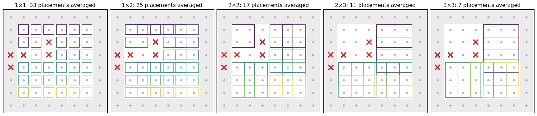
Cell berikutnya menunjukkan penempatan tiap bentuk yang masuk ke rata-rata di bawah: setiap penempatan di bagian bulk lattice tanpa site yang ditandai (tanda silang merah). Penempatan yang menyentuh tepi (diarsir) dikeluarkan. Qubit tepi punya lebih sedikit bond, jadi mengacak lebih lambat. Jika dirata-rata sendiri, mereka melakukan crossover satu langkah penuh lebih lambat daripada penempatan bulk, untuk setiap bentuk dan metode. Setiap penempatan yang dirata-rata punya box-nya sendiri, diberi warna menurut penempatan.
def touches_edge(qubits):
    # Whether a placement includes a site on the edge of the lattice
    return any(
        q % num_cols_hw in (0, num_cols_hw - 1)
        or q // num_cols_hw in (0, num_rows_hw - 1)
        for q in qubits
    )

# The placements of each shape that enter the averages: in the bulk, and without a flagged site
kept_placements = {
    label: [
        k
        for k, qubits in enumerate(patch_list)
        if not touches_edge(qubits) and not set(qubits) & flagged
    ]
    for label, patch_list in positions.items()
}
placement_cmap = plt.get_cmap("viridis")
fig, axes = plt.subplots(
    1, len(positions), figsize=(17, 4.4), layout="constrained"
)
for ax, (label, patch_list) in zip(axes, positions.items()):
    width, height = patch_shapes[label]
    for q in range(num_qubits_hw):
        x, y = q % num_cols_hw, q // num_cols_hw
        if touches_edge([q]):  # shade the edge of the lattice
            ax.add_patch(
                plt.Rectangle(
                    (x - 0.5, y - 0.5), 1, 1, color="0.92", zorder=0
                )
            )
        ax.plot(x, y, "o", color="0.7", ms=4, zorder=1)
    kept = kept_placements[label]
    for i, k in enumerate(kept):
        qubits = patch_list[k]
        x0, y0 = (
            qubits[0] % num_cols_hw,
            qubits[0] // num_cols_hw,
        )  # top-left site of the placement
        ax.add_patch(
            plt.Rectangle(
                (x0 - 0.4, y0 - 0.4),
                width - 0.2,
                height - 0.2,
                fill=False,
                lw=1.2,
                ec=placement_cmap(i / max(len(kept) - 1, 1)),
                zorder=2,
            )
        )
    for q in flagged:
        ax.plot(
            q % num_cols_hw,
            q // num_cols_hw,
            "x",
            color="#d62728",
            ms=11,
            mew=3,
            zorder=3,
        )
    ax.set_xlim(-0.6, num_cols_hw - 0.4)
    ax.set_ylim(num_rows_hw - 0.4, -0.6)
    ax.set_aspect("equal")
    ax.set_xticks([])
    ax.set_yticks([])
    ax.set_title(f"{label}: {len(kept)} placements averaged")
plt.show()
PEA
Metode ketiga tidak butuh referensi klasik. Untuk setiap paritas, ambil nilai pada faktor noise 1, 1,5, dan 2, bagi dengan peredaman readout yang dipelajari (TREX), fit eksponensial terhadap faktor noise, dan ekstrapolasi ke noise nol. Paritas yang berganti tanda atau hampir nol memakai fit garis lurus. Mengurangi varians butuh estimasi varians yang andal, yang mudah untuk paritas mentah dan terskala tetapi tidak untuk keluaran fit nonlinear dengan clipping dan fallback. Karena itu PEA memakai cara standar lain untuk menghilangkan bias kuadrat. Ekstrapolasikan tiap separuh randomisasi secara terpisah dan kalikan kedua estimasi independen itu.
def readout_fidelity(support):
    # Damping of <Z_S> by the learned readout noise
    pauli = QubitSparsePauli.from_sparse_label(
        ("Z" * len(support), list(support)), num_qubits_hw
    )
    return readout_map.pauli_fidelity(pauli)

def extrapolate_to_zero(values):
    # Fit a * exp(b * factor) to each column of values (noise factors first), or a line
    # where the values change sign or come within 1e-3 of zero
    result = np.polynomial.polynomial.polyfit(noise_factors, values, 1)[0]
    sign = np.sign(values[0])
    usable = np.all(np.sign(values) == sign, axis=0) & (
        np.abs(values).min(axis=0) > 1e-3
    )
    if usable.any():
        log_fit = np.polynomial.polynomial.polyfit(
            noise_factors, np.log(np.abs(values[:, usable])), 1
        )
        result[usable] = sign[usable] * np.exp(log_fit[0])
    return result

def pea_ipr(parities, fidelities, num_patch):
    # parities has shape (noise factors, randomizations, supports). Extrapolate the two
    # halves of the randomizations separately; their errors are independent, so the
    # product of the two estimates of each parity has no shot-noise bias
    def zero_noise(p):
        # A parity cannot exceed 1 in magnitude, so cap the extrapolated values there
        return np.clip(
            extrapolate_to_zero(p.mean(axis=1) / fidelities), -1, 1
        )

    half = parities.shape[1] // 2
    first, second = (
        zero_noise(parities[:, :half]),
        zero_noise(parities[:, half:]),
    )
    return float((1 + np.dot(first, second)) / 2**num_patch)
Keempat estimasi, dan crossover-nya
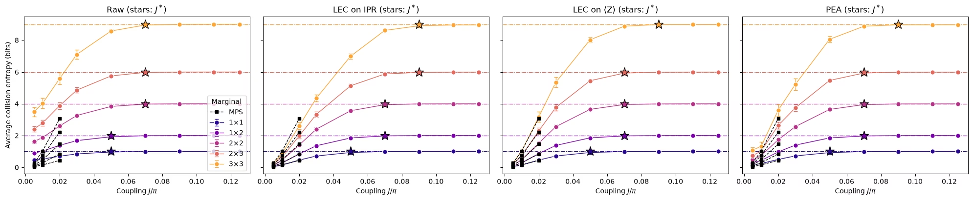
Fungsi berikutnya menghitung estimasi mentah, LEC-pada-IPR, LEC-pada-, dan PEA dari IPR satu posisi marginal pada setiap coupling. Fungsi ini juga mengestimasi shot noise masing-masing, dengan bootstrapping atas randomisasi. Cell menjalankannya untuk setiap penempatan yang masuk ke rata-rata, yang butuh sekitar satu setengah menit.
def estimate_iprs(qubits, key):
    # Raw, LEC-on-IPR, LEC-on-<Z>, and PEA IPRs of one marginal position at every coupling,
    # with the shot noise of each from a bootstrap over the randomizations
    n = len(qubits)
    supports = parity_supports(qubits)
    # Parities with shape (noise factors, randomizations, supports), per coupling
    parities = [
        np.stack([parity_expectation_values(b, supports) for b in bits])
        for bits in raw_bits
    ]
    patch_bits = [
        bits[0][:, :, qubits] for bits in raw_bits
    ]  # noise factor 1
    values, errors = lec_estimates(
        patch_bits,
        [p[0] for p in parities],
        references[(calibration_hw, 64)][key],
        calibration_hw,
        n,
    )
    fidelities = np.array([readout_fidelity(s) for s in supports])

    def pea_statistic(p):
        return pea_ipr(p, fidelities, n)

    values["raw"] = [ipr_from_shots(b) for b in patch_bits]
    errors["raw"] = [bootstrap_error(ipr_from_shots, b) for b in patch_bits]
    values["PEA"] = [pea_statistic(p) for p in parities]
    errors["PEA"] = [
        bootstrap_error(pea_statistic, p, axis=1) for p in parities
    ]  # randomizations are axis 1
    return {m: np.array(v) for m, v in values.items()}, {
        m: np.array(e) for m, e in errors.items()
    }

methods = ["LEC on IPR", "LEC on ⟨Z⟩", "PEA"]
method_colors = {
    "LEC on IPR": "#2a78d6",
    "LEC on ⟨Z⟩": "#1baf7a",
    "PEA": "#eb6834",
}
iprs, ipr_errors = {}, {}
for label, patch_list in positions.items():
    for k in kept_placements[label]:
        iprs[label, k], ipr_errors[label, k] = estimate_iprs(
            patch_list[k], f"{label} {k}"
        )
print(f"{len(iprs)} clean marginal positions")
93 clean marginal positions
def crossover_coupling(couplings, entropies, haar, tolerance=0.1):
    # Smallest coupling whose entropy is within tolerance of the random-state value
    for coupling, entropy in zip(couplings, entropies):
        if entropy >= haar - tolerance:
            return coupling
    return None

def reference_ipr(index, chi, key):
    # IPR of the MPS distribution of a marginal
    return float((references[(index, chi)][key] ** 2).sum())

mps_settings = [
    (calibration_hw, 64),
    (1, 128),
    (2, 128),
]  # (coupling index, bond dimension)
panels = ["raw", *methods]

# Average IPR of every shape over its clean placements, then the entropy and the crossover
hw_entropies = {
    method: {} for method in panels
}  # per method and shape: average entropy and its error
crossovers = {method: {} for method in panels}
mps_entropies = {}  # per shape: MPS entropy, averaged over the same placements, at mps_settings
for label, patch_list in positions.items():
    haar = haar_entropy(len(patch_list[0]), num_qubits_hw)
    keys = [(shape, k) for (shape, k) in iprs if shape == label]
    mps_entropies[label] = [
        collision_entropy(
            np.mean([reference_ipr(j, chi, f"{label} {k}") for _, k in keys])
        )
        for j, chi in mps_settings
    ]
    for method in panels:
        ipr, ipr_error = average_ipr(
            [iprs[key][method] for key in keys],
            [ipr_errors[key][method] for key in keys],
        )
        entropy = collision_entropy(ipr)
        hw_entropies[method][label] = (entropy, ipr_error / (ipr * np.log(2)))
        crossovers[method][label] = crossover_coupling(
            couplings_hw, entropy, haar
        )
fig, axes = plt.subplots(
    1, len(panels), figsize=(5 * len(panels), 4.2), sharey=True
)
for (label, patch_list), color in zip(positions.items(), colors):
    haar = haar_entropy(len(patch_list[0]), num_qubits_hw)
    for ax, method in zip(axes, panels):
        entropy, error = hw_entropies[method][label]
        ax.errorbar(
            couplings_hw / np.pi,
            entropy,
            yerr=error,
            fmt="o-",
            color=color,
            mec="white",
            ms=7,
            lw=1,
            capsize=3,
            label=label,
        )
        ax.plot(
            couplings_hw[[j for j, _ in mps_settings]] / np.pi,
            mps_entropies[label],
            "s--",
            color="black",
            ms=4,
            lw=1,
            label="MPS" if label == "3×3" else None,
            zorder=4,
        )
        ax.axhline(haar, color=color, ls="dashdot", lw=0.9)
        if crossovers[method][label]:
            ax.plot(
                crossovers[method][label] / np.pi,
                haar,
                "*",
                ms=14,
                color=color,
                mec="black",
                zorder=3,
            )
for ax, method in zip(axes, panels):
    ax.set_title(f"{'Raw' if method == 'raw' else method} (stars: $J^*$)")
    ax.set_xlabel("Coupling $J/\\pi$")
axes[0].set_ylabel("Average collision entropy (bits)")
axes[0].legend(title="Marginal", loc="lower right")
fig.tight_layout()
plt.show()
Penutup
Yang dibutuhkan untuk menjalankan eksperimen sebesar ini:
-
Circuit yang strukturnya tidak bergantung pada , dikompilasi satu sublayer pada satu waktu, sehingga satu model noise melayani seluruh sweep.
-
Estimator yang bekerja dari bitstring: penghitungan pasangan untuk IPR sebuah marginal, dan bentuk Parseval, dengan varians dikurangkan dari tiap paritas kuadrat, ketika inputnya adalah nilai ekspektasi yang sudah dimitigasi.
-
Jangkar klasik yang murah: state ideal pada kecil mengalibrasi noise, dan coupling held-out menguji kalibrasinya. Mengalibrasi tiap secara terpisah, bukan IPR secara keseluruhan, adalah yang membuat marginal besar cocok.
-
Tool IBM untuk pekerjaan berat: box dan twirling Samplomatic,
NoiseLearnerV3, dynamical decoupling, dan satu jobExecutordengan amplifikasi noise untuk PEA. -
Pemeriksaan kualitas data yang hanya memakai data.
Langkah berikutnya. Untuk mendalami mitigasi, lihat tutorial probabilistic error amplification dan PEC with shaded lightcones.