Metode kompilasi untuk sirkuit simulasi Hamiltonian
Estimasi penggunaan: kurang dari 1 menit pada prosesor IBM Heron (CATATAN: Ini hanya estimasi. Waktu eksekusi kamu bisa berbeda.)
Hasil pembelajaran
Setelah menyelesaikan tutorial ini, kamu akan memahami:
- Cara menggunakan transpiler Qiskit dengan SABRE untuk optimasi layout dan routing
- Cara memanfaatkan transpiler bertenaga AI untuk optimasi sirkuit tingkat lanjut
- Cara menggunakan plugin Rustiq untuk mensintesis operasi
PauliEvolutionGatepada sirkuit simulasi Hamiltonian - Cara melakukan benchmark dan membandingkan metode kompilasi menggunakan kedalaman dua-Qubit, jumlah gate total, dan waktu eksekusi
Prasyarat
Kami sarankan kamu sudah familiar dengan topik-topik berikut sebelum menjalani tutorial ini:
Latar belakang
Kompilasi sirkuit kuantum mengubah algoritma kuantum tingkat tinggi menjadi sirkuit fisik yang mematuhi batasan perangkat keras target. Kompilasi yang efektif dapat secara signifikan mengurangi kedalaman sirkuit dan jumlah gate, yang keduanya berdampak langsung pada kualitas hasil di perangkat kuantum near-term.
Tutorial ini melakukan benchmark tiga metode kompilasi pada sirkuit simulasi Hamiltonian yang dibangun dengan PauliEvolutionGate. Sirkuit-sirkuit ini memodelkan interaksi berpasangan antar qubit (seperti suku , , dan ) dan umum digunakan dalam kimia kuantum, fisika materi terkondensasi, dan ilmu material.
Sirkuit benchmark berasal dari koleksi Hamlib, yang diakses melalui repositori Benchpress. Hamlib menyediakan sekumpulan Hamiltonian representatif yang terstandarisasi, sehingga memungkinkan perbandingan strategi kompilasi pada beban kerja simulasi yang realistis.
Gambaran umum metode kompilasi
Transpiler Qiskit dengan SABRE
Transpiler Qiskit menggunakan algoritma SABRE (SWAP-based BidiREctional heuristic search) untuk mengoptimalkan layout dan routing sirkuit. SABRE berfokus pada minimalisasi gate SWAP dan dampaknya pada kedalaman sirkuit sambil mematuhi batasan konektivitas perangkat keras. Ini adalah metode serbaguna yang memberikan keseimbangan antara performa dan waktu kompilasi. Untuk detail lebih lanjut, lihat [1]. Keunggulan dan eksplorasi parameter SABRE dibahas secara mendalam dalam tutorial terpisah.
Transpiler bertenaga AI
Transpiler bertenaga AI menggunakan machine learning untuk memprediksi strategi transpilasi optimal dengan menganalisis pola dalam struktur sirkuit dan batasan perangkat keras. Ia juga dapat menerapkan pass AIPauliNetworkSynthesis, yang menargetkan sirkuit jaringan Pauli menggunakan pendekatan sintesis berbasis reinforcement learning. Untuk informasi lebih lanjut, lihat [2] dan [3].
Plugin Rustiq
Plugin Rustiq menyediakan teknik sintesis canggih khusus untuk operasi PauliEvolutionGate, yang merepresentasikan rotasi Pauli yang umum digunakan dalam dinamika Trotterisasi. Plugin ini dirancang untuk menghasilkan dekomposisi sirkuit berkedalaman rendah untuk beban kerja simulasi Hamiltonian. Untuk detail lebih lanjut, lihat [4].
Metrik utama
Kami membandingkan ketiga metode pada metrik-metrik berikut:
- Kedalaman dua-Qubit: Kedalaman sirkuit yang hanya menghitung gate dua-Qubit. Ini sering menjadi hambatan fidelitas pada perangkat keras nyata.
- Ukuran sirkuit (jumlah gate total): Jumlah total gate dalam sirkuit yang sudah ditranspilasi.
- Waktu eksekusi: Waktu clock untuk transpilasi.
Persyaratan
Sebelum memulai tutorial ini, pastikan kamu sudah menginstal yang berikut:
- Qiskit SDK v2.0 atau lebih baru, dengan dukungan visualisasi
- Qiskit Runtime v0.22 atau lebih baru (
pip install qiskit-ibm-runtime) - Qiskit Aer (
pip install qiskit-aer) - Qiskit IBM Transpiler (
pip install qiskit-ibm-transpiler) - Mode lokal transpiler AI Qiskit (
pip install qiskit_ibm_ai_local_transpiler) - Networkx (
pip install networkx)
Pengaturan
# Added by doQumentation — required packages for this notebook
!pip install -q matplotlib numpy qiskit qiskit-aer qiskit-ibm-runtime qiskit-ibm-transpiler requests scipy
from qiskit.circuit import QuantumCircuit
from qiskit_ibm_runtime import QiskitRuntimeService, SamplerV2
from qiskit.circuit.library import PauliEvolutionGate
from qiskit_ibm_transpiler import generate_ai_pass_manager
from qiskit.quantum_info import SparsePauliOp
from qiskit.transpiler.preset_passmanagers import generate_preset_pass_manager
from qiskit.transpiler.passes.synthesis.high_level_synthesis import HLSConfig
from qiskit_aer import AerSimulator
from qiskit_aer.noise import NoiseModel, depolarizing_error
from collections import Counter
from statistics import mean, stdev
from scipy.sparse import SparseEfficiencyWarning
import time
import warnings
import matplotlib.pyplot as plt
import matplotlib.ticker as ticker
import numpy as np
import json
import requests
import logging

# Suppress noisy loggers and warnings
logging.getLogger(
    "qiskit_ibm_transpiler.wrappers.ai_local_synthesis"
).setLevel(logging.ERROR)
warnings.filterwarnings("ignore", category=FutureWarning)
warnings.filterwarnings("ignore", category=SparseEfficiencyWarning)

seed = 42  # Seed for reproducibility
Sambungkan ke backend
Pilih backend yang akan digunakan untuk contoh skala kecil maupun skala besar. Backend menentukan coupling map dan basis gate yang menjadi target transpiler.
# QiskitRuntimeService.save_account(channel="ibm_quantum_platform",
# token="<YOUR-API-KEY>", overwrite=True, set_as_default=True)
service = QiskitRuntimeService(channel="ibm_quantum_platform")
backend = service.least_busy(operational=True, simulator=False)
print(f"Using backend: {backend.name}")
Using backend: ibm_pittsburgh
Definisikan pass manager
Siapkan tiga metode kompilasi.
# SABRE pass manager (Qiskit default at optimization level 3)
pm_sabre = generate_preset_pass_manager(
    optimization_level=3, backend=backend, seed_transpiler=seed
)
# AI transpiler pass manager (local mode)
pm_ai = generate_ai_pass_manager(
    backend=backend, optimization_level=3, ai_optimization_level=3
)
Fetching 127 files: 0%| | 0/127 [00:00<?, ?it/s]
# Rustiq pass manager for PauliEvolutionGate synthesis
hls_config = HLSConfig(
    PauliEvolution=[
        (
            "rustiq",
            {
                "nshuffles": 400,
                "upto_phase": True,
                "fix_clifford": True,
                "preserve_order": False,
                "metric": "depth",
            },
        )
    ]
)
pm_rustiq = generate_preset_pass_manager(
    optimization_level=3,
    backend=backend,
    hls_config=hls_config,
    seed_transpiler=seed,
)
Definisikan fungsi pembantu
Fungsi berikut mentranspilasi daftar sirkuit menggunakan pass manager yang diberikan, dan mencatat metrik utama (kedalaman dua-Qubit, ukuran sirkuit, dan waktu eksekusi) untuk setiap sirkuit.
def capture_transpilation_metrics(
    results, pass_manager, circuits, method_name
):
    """
    Transpile circuits and append one metrics record per circuit to
    ``results``.

    Args:
        results (list): List of dicts to append the metrics records to.
        pass_manager: Pass manager used for transpilation.
        circuits (list): List of quantum circuits to transpile.
        method_name (str): Name of the transpilation method.

    Returns:
        list: List of transpiled circuits.
    """
    transpiled_circuits = []

    for i, qc in enumerate(circuits):
        start_time = time.time()
        transpiled_qc = pass_manager.run(qc)
        end_time = time.time()

        # Decompose swaps for consistency across methods
        transpiled_qc = transpiled_qc.decompose(gates_to_decompose=["swap"])

        transpilation_time = end_time - start_time
        two_qubit_depth = transpiled_qc.depth(
            lambda x: x.operation.num_qubits == 2
        )
        circuit_size = transpiled_qc.size()

        results.append(
            {
                "method": method_name,
                "qc_name": qc.name,
                "qc_index": i,
                "num_qubits": qc.num_qubits,
                "two_qubit_depth": two_qubit_depth,
                "size": circuit_size,
                "runtime": transpilation_time,
            }
        )
        transpiled_circuits.append(transpiled_qc)
        print(
            f"[{method_name}] Circuit {i} ({qc.name}): "
            f"2Q depth={two_qubit_depth}, size={circuit_size}, "
            f"time={transpilation_time:.2f}s"
        )

    return transpiled_circuits
def _method_order(results):
    """Return the distinct method names in their first-seen order."""
    order = []
    for r in results:
        if r["method"] not in order:
            order.append(r["method"])
    return order

def print_summary_table(results):
    """
    Print the mean and standard deviation of each metric per compilation
    method, followed by the mean percent improvement relative to SABRE.
    """
    metrics = [
        ("two_qubit_depth", "2Q Depth"),
        ("size", "Gate Count"),
        ("runtime", "Runtime (s)"),
    ]
    methods = _method_order(results)
    by_method = {m: [r for r in results if r["method"] == m] for m in methods}
    sabre_by_index = {r["qc_index"]: r for r in by_method.get("SABRE", [])}

    col_w = 22
    name_w = max(len(m) for m in methods)
    header = f"{'Method':<{name_w}}" + "".join(
        f"  {label:>{col_w}}" for _, label in metrics
    )

    print("Mean +/- std per compilation method")
    print(header)
    print("-" * len(header))
    for method in methods:
        cells = []
        for key, _ in metrics:
            values = [r[key] for r in by_method[method]]
            std = stdev(values) if len(values) > 1 else 0.0
            cells.append(f"{mean(values):,.1f} +/- {std:,.1f}")
        print(
            f"{method:<{name_w}}" + "".join(f"  {c:>{col_w}}" for c in cells)
        )

    others = [m for m in methods if m != "SABRE"]
    if others and sabre_by_index:
        print()
        print("Mean % improvement vs SABRE (positive = better than SABRE)")
        print(header)
        print("-" * len(header))
        for method in others:
            cells = []
            for key, _ in metrics:
                pct = [
                    (sabre_by_index[r["qc_index"]][key] - r[key])
                    / sabre_by_index[r["qc_index"]][key]
                    * 100
                    for r in by_method[method]
                    if sabre_by_index.get(r["qc_index"])
                    and sabre_by_index[r["qc_index"]][key]
                ]
                if pct:
                    std = stdev(pct) if len(pct) > 1 else 0.0
                    cells.append(f"{mean(pct):+.1f}% +/- {std:.1f}%")
                else:
                    cells.append("n/a")
            print(
                f"{method:<{name_w}}"
                + "".join(f"  {c:>{col_w}}" for c in cells)
            )
def print_per_circuit_comparison(results, num_rows=5):
    """
    Print a per-metric comparison of the compilation methods for the
    first ``num_rows`` circuits (sorted by qubit count). The best
    (lowest) value for each metric is marked with an asterisk.
    """
    metrics = [
        ("two_qubit_depth", "2Q Depth"),
        ("size", "Gate Count"),
        ("runtime", "Runtime (s)"),
    ]
    methods = _method_order(results)

    by_index = {}
    for r in results:
        by_index.setdefault(r["qc_index"], {})[r["method"]] = r
    ordered = sorted(
        by_index.items(),
        key=lambda kv: (next(iter(kv[1].values()))["num_qubits"], kv[0]),
    )[:num_rows]

    for key, label in metrics:
        print(f"{label} (first {num_rows} circuits by qubit count); * = best")
        header = f"{'Idx':>3}  {'Circuit':<16} {'Q':>3}" + "".join(
            f"{m:>9}" for m in methods
        )
        print(header)
        print("-" * len(header))
        for idx, method_map in ordered:
            any_record = next(iter(method_map.values()))
            present = {
                m: method_map[m][key] for m in methods if m in method_map
            }
            best = min(present.values())
            line = (
                f"{idx:>3}  {any_record['qc_name'][:16]:<16} "
                f"{any_record['num_qubits']:>3}"
            )
            for m in methods:
                value = method_map[m][key]
                text = f"{value:.2f}" if key == "runtime" else f"{int(value)}"
                if value == best:
                    text += "*"
                line += f"{text:>9}"
            print(line)
        print()
Muat sirkuit Hamiltonian dari Hamlib
Kami memuat sekumpulan Hamiltonian representatif dari repositori Benchpress dan membangun sirkuit PauliEvolutionGate. Sirkuit yang melebihi jumlah Qubit backend dihapus, bersama sirkuit yang ukuran dekomposisinya melebihi 1.500 gate (untuk menjaga waktu transpilasi tetap wajar).
# Obtain the Hamiltonian JSON from the benchpress repository
url = "https://raw.githubusercontent.com/Qiskit/benchpress/e7b29ef7be4cc0d70237b8fdc03edbd698908eff/benchpress/hamiltonian/hamlib/100_representative.json"
response = requests.get(url)
response.raise_for_status()
ham_records = json.loads(response.text)

# Remove circuits that are too large for the backend
ham_records = [
    h for h in ham_records if h["ham_qubits"] <= backend.num_qubits
]

# Build PauliEvolutionGate circuits
qc_ham_list = []
for h in ham_records:
    terms = h["ham_hamlib_hamiltonian_terms"]
    coeff = h["ham_hamlib_hamiltonian_coefficients"]
    num_qubits = h["ham_qubits"]
    name = h["ham_problem"]

    evo_gate = PauliEvolutionGate(SparsePauliOp(terms, coeff))
    qc = QuantumCircuit(num_qubits)
    qc.name = name
    qc.append(evo_gate, range(num_qubits))
    qc_ham_list.append(qc)

# Remove circuits whose decomposed size exceeds 1500 gates so that transpilation completes in a reasonable time frame
qc_ham_list = [qc for qc in qc_ham_list if qc.decompose().size() <= 1500]

print(f"Total Hamiltonian circuits loaded: {len(qc_ham_list)}")
print(
    f"Qubit range: {min(qc.num_qubits for qc in qc_ham_list)} to {max(qc.num_qubits for qc in qc_ham_list)}"
)
Total Hamiltonian circuits loaded: 42
Qubit range: 2 to 112
Bagi sirkuit menjadi kelompok skala kecil (kurang dari 20 Qubit) dan skala besar (20 Qubit atau lebih).
qc_small = [qc for qc in qc_ham_list if qc.num_qubits < 20]
qc_large = [qc for qc in qc_ham_list if qc.num_qubits >= 20]

print(f"Small-scale circuits (<20 qubits): {len(qc_small)}")
print(f"Large-scale circuits (>=20 qubits): {len(qc_large)}")
Small-scale circuits (<20 qubits): 20
Large-scale circuits (>=20 qubits): 22
Pratinjau salah satu sirkuit Hamiltonian skala kecil sebelum transpilasi.
# We decompose the circuit here, otherwise it would just be a PauliEvolutionGate box,
# which isn't very informative to look at!
qc_small[0].decompose().draw("mpl", fold=-1)

Contoh skala kecil
Di bagian ini, kami melakukan benchmark tiga metode kompilasi pada sirkuit Hamiltonian dengan kurang dari 20 Qubit. Sirkuit-sirkuit ini ditranspilasi dengan cepat dan memberikan gambaran jelas tentang cara setiap metode menangani sirkuit dengan kompleksitas sedang.
Langkah 1: Petakan input klasik ke masalah kuantum
Setiap Hamiltonian dikodekan sebagai sirkuit PauliEvolutionGate. Sirkuit-sirkuit ini sudah dibangun di bagian pengaturan dari data benchmark Hamlib.
Langkah 2: Optimasi masalah untuk eksekusi perangkat keras kuantum
Kami mentranspilasi semua sirkuit skala kecil menggunakan masing-masing dari tiga pass manager, lalu mengumpulkan metriknya.
results_small = []

tqc_sabre_small = capture_transpilation_metrics(
    results_small, pm_sabre, qc_small, "SABRE"
)
tqc_ai_small = capture_transpilation_metrics(
    results_small, pm_ai, qc_small, "AI"
)
tqc_rustiq_small = capture_transpilation_metrics(
    results_small, pm_rustiq, qc_small, "Rustiq"
)
[SABRE] Circuit 0 (all-vib-bh): 2Q depth=3, size=30, time=2.09s
[SABRE] Circuit 1 (all-vib-c2h): 2Q depth=18, size=111, time=0.01s
[SABRE] Circuit 2 (all-vib-o3): 2Q depth=6, size=58, time=0.00s
[SABRE] Circuit 3 (all-vib-c2h): 2Q depth=2, size=37, time=0.01s
[SABRE] Circuit 4 (graph-gnp_k-2): 2Q depth=24, size=126, time=0.01s
[SABRE] Circuit 5 (LiH): 2Q depth=66, size=285, time=0.01s
[SABRE] Circuit 6 (all-vib-fccf): 2Q depth=66, size=339, time=0.01s
[SABRE] Circuit 7 (all-vib-ch2): 2Q depth=88, size=413, time=0.01s
[SABRE] Circuit 8 (all-vib-f2): 2Q depth=180, size=1000, time=0.02s
[SABRE] Circuit 9 (all-vib-bhf2): 2Q depth=18, size=223, time=0.03s
[SABRE] Circuit 10 (graph-gnp_k-4): 2Q depth=122, size=675, time=0.02s
[SABRE] Circuit 11 (Be2): 2Q depth=343, size=1628, time=0.03s
[SABRE] Circuit 12 (all-vib-fccf): 2Q depth=14, size=134, time=0.00s
[SABRE] Circuit 13 (uf20-ham): 2Q depth=50, size=341, time=0.01s
[SABRE] Circuit 14 (TSP_Ncity-4): 2Q depth=118, size=615, time=0.01s
[SABRE] Circuit 15 (graph-complete_bipart): 2Q depth=232, size=1420, time=0.03s
[SABRE] Circuit 16 (all-vib-cyclo_propene): 2Q depth=18, size=354, time=0.93s
[SABRE] Circuit 17 (all-vib-hno): 2Q depth=6, size=174, time=0.14s
[SABRE] Circuit 18 (all-vib-fccf): 2Q depth=30, size=286, time=0.01s
[SABRE] Circuit 19 (tfim): 2Q depth=31, size=232, time=0.03s
[AI] Circuit 0 (all-vib-bh): 2Q depth=3, size=30, time=0.01s
Fetching 4 files: 0%| | 0/4 [00:00<?, ?it/s]
[AI] Circuit 1 (all-vib-c2h): 2Q depth=18, size=101, time=0.18s
[AI] Circuit 2 (all-vib-o3): 2Q depth=6, size=58, time=0.01s
[AI] Circuit 3 (all-vib-c2h): 2Q depth=2, size=37, time=0.01s
[AI] Circuit 4 (graph-gnp_k-2): 2Q depth=24, size=133, time=0.07s
[AI] Circuit 5 (LiH): 2Q depth=62, size=267, time=8.00s
[AI] Circuit 6 (all-vib-fccf): 2Q depth=65, size=300, time=0.18s
[AI] Circuit 7 (all-vib-ch2): 2Q depth=79, size=353, time=0.16s
[AI] Circuit 8 (all-vib-f2): 2Q depth=176, size=998, time=0.43s
[AI] Circuit 9 (all-vib-bhf2): 2Q depth=18, size=194, time=0.11s
[AI] Circuit 10 (graph-gnp_k-4): 2Q depth=114, size=668, time=0.18s
[AI] Circuit 11 (Be2): 2Q depth=292, size=1382, time=0.88s
[AI] Circuit 12 (all-vib-fccf): 2Q depth=14, size=134, time=0.01s
[AI] Circuit 13 (uf20-ham): 2Q depth=40, size=330, time=0.16s
[AI] Circuit 14 (TSP_Ncity-4): 2Q depth=96, size=600, time=0.29s
[AI] Circuit 15 (graph-complete_bipart): 2Q depth=231, size=1531, time=0.46s
[AI] Circuit 16 (all-vib-cyclo_propene): 2Q depth=18, size=309, time=0.25s
[AI] Circuit 17 (all-vib-hno): 2Q depth=10, size=198, time=0.15s
[AI] Circuit 18 (all-vib-fccf): 2Q depth=34, size=402, time=0.02s
[AI] Circuit 19 (tfim): 2Q depth=44, size=311, time=0.15s
[Rustiq] Circuit 0 (all-vib-bh): 2Q depth=3, size=30, time=0.01s
[Rustiq] Circuit 1 (all-vib-c2h): 2Q depth=13, size=69, time=0.00s
[Rustiq] Circuit 2 (all-vib-o3): 2Q depth=13, size=82, time=0.01s
[Rustiq] Circuit 3 (all-vib-c2h): 2Q depth=2, size=40, time=0.01s
[Rustiq] Circuit 4 (graph-gnp_k-2): 2Q depth=31, size=132, time=0.01s
[Rustiq] Circuit 5 (LiH): 2Q depth=59, size=285, time=0.01s
[Rustiq] Circuit 6 (all-vib-fccf): 2Q depth=34, size=193, time=0.00s
[Rustiq] Circuit 7 (all-vib-ch2): 2Q depth=49, size=302, time=0.01s
[Rustiq] Circuit 8 (all-vib-f2): 2Q depth=141, size=807, time=0.02s
[Rustiq] Circuit 9 (all-vib-bhf2): 2Q depth=13, size=146, time=0.02s
[Rustiq] Circuit 10 (graph-gnp_k-4): 2Q depth=129, size=683, time=0.02s
[Rustiq] Circuit 11 (Be2): 2Q depth=220, size=1101, time=0.02s
[Rustiq] Circuit 12 (all-vib-fccf): 2Q depth=53, size=333, time=0.01s
[Rustiq] Circuit 13 (uf20-ham): 2Q depth=63, size=425, time=0.01s
[Rustiq] Circuit 14 (TSP_Ncity-4): 2Q depth=123, size=767, time=0.02s
[Rustiq] Circuit 15 (graph-complete_bipart): 2Q depth=309, size=2107, time=0.05s
[Rustiq] Circuit 16 (all-vib-cyclo_propene): 2Q depth=16, size=283, time=0.32s
[Rustiq] Circuit 17 (all-vib-hno): 2Q depth=19, size=291, time=0.32s
[Rustiq] Circuit 18 (all-vib-fccf): 2Q depth=44, size=546, time=0.02s
[Rustiq] Circuit 19 (tfim): 2Q depth=24, size=416, time=0.01s
Tabel di bawah merangkum rata-rata dan deviasi standar setiap metrik di seluruh sirkuit skala kecil, beserta persentase peningkatan relatif terhadap SABRE. Karena ukuran sirkuit sangat bervariasi, deviasi standar memberikan konteks penting untuk menginterpretasikan rata-rata tersebut.
print_summary_table(results_small)
Mean +/- std per compilation method
Method                2Q Depth              Gate Count             Runtime (s)
------------------------------------------------------------------------------
SABRE            71.8 +/- 89.6         424.1 +/- 446.0             0.2 +/- 0.5
AI               67.3 +/- 80.2         416.8 +/- 426.7             0.6 +/- 1.8
Rustiq           67.9 +/- 80.0         451.9 +/- 484.7             0.0 +/- 0.1

Mean % improvement vs SABRE (positive = better than SABRE)
Method                2Q Depth              Gate Count             Runtime (s)
------------------------------------------------------------------------------
AI             -2.1% +/- 19.8%         -0.6% +/- 14.7%   -5635.1% +/- 20725.2%
Rustiq        -25.3% +/- 85.4%        -16.3% +/- 50.4%         -7.0% +/- 60.6%
Tabel per-sirkuit menunjukkan perbandingan setiap metode pada sirkuit individual. Nilai terbaik untuk setiap metrik ditandai dengan tanda bintang. Perhatikan bahwa untuk sirkuit paling sederhana, ketiga metode sering mencapai hasil yang sama.
print_per_circuit_comparison(results_small, num_rows=8)
2Q Depth (first 8 circuits by qubit count); * = best
Idx  Circuit            Q    SABRE       AI   Rustiq
----------------------------------------------------
  0  all-vib-bh         2       3*       3*       3*
  1  all-vib-c2h        3       18       18      13*
  2  all-vib-o3         4       6*       6*       13
  3  all-vib-c2h        4       2*       2*       2*
  4  graph-gnp_k-2      4      24*      24*       31
  5  LiH                4       66       62      59*
  6  all-vib-fccf       4       66       65      34*
  7  all-vib-ch2        4       88       79      49*

Gate Count (first 8 circuits by qubit count); * = best
Idx  Circuit            Q    SABRE       AI   Rustiq
----------------------------------------------------
  0  all-vib-bh         2      30*      30*      30*
  1  all-vib-c2h        3      111      101      69*
  2  all-vib-o3         4      58*      58*       82
  3  all-vib-c2h        4      37*      37*       40
  4  graph-gnp_k-2      4     126*      133      132
  5  LiH                4      285     267*      285
  6  all-vib-fccf       4      339      300     193*
  7  all-vib-ch2        4      413      353     302*

Runtime (s) (first 8 circuits by qubit count); * = best
Idx  Circuit            Q    SABRE       AI   Rustiq
----------------------------------------------------
  0  all-vib-bh         2     2.09     0.01    0.01*
  1  all-vib-c2h        3     0.01     0.18    0.00*
  2  all-vib-o3         4    0.00*     0.01     0.01
  3  all-vib-c2h        4     0.01     0.01    0.01*
  4  graph-gnp_k-2      4    0.01*     0.07     0.01
  5  LiH                4    0.01*     8.00     0.01
  6  all-vib-fccf       4     0.01     0.18    0.00*
  7  all-vib-ch2        4     0.01     0.16    0.01*
Visualisasi hasil
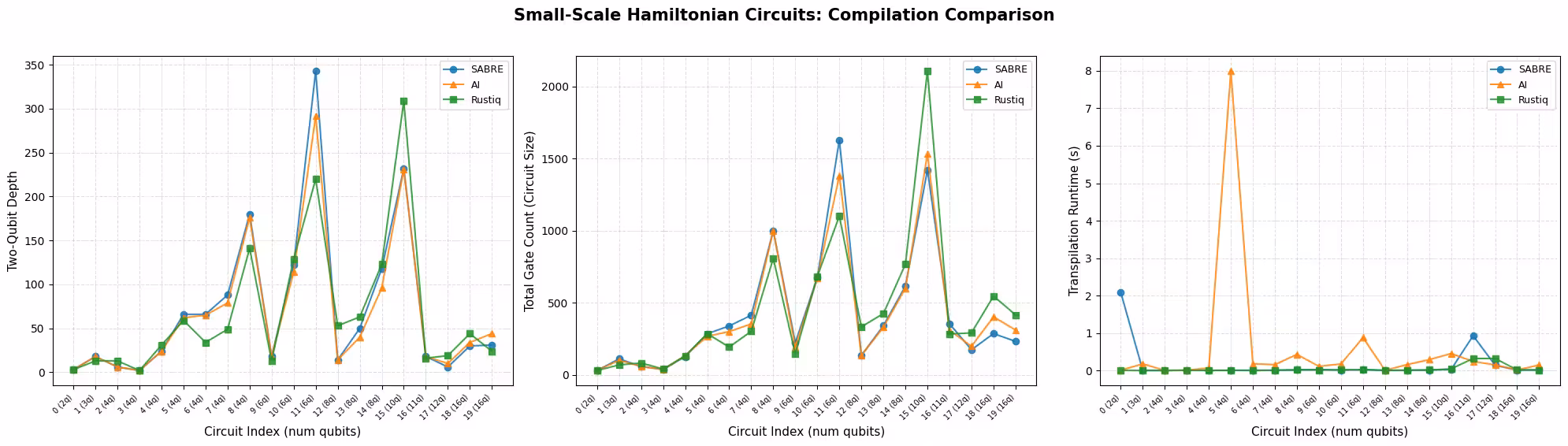
Plot di bawah membandingkan ketiga metode pada setiap metrik secara per-sirkuit. Sirkuit diurutkan berdasarkan jumlah Qubit dan diberi label berdasarkan indeks pada sumbu-x, karena beberapa sirkuit bisa memiliki jumlah Qubit yang sama.
def plot_transpilation_comparison(results, title_prefix):
    """
    Create a three-panel figure comparing compilation methods on
    two-qubit depth, circuit size, and runtime.

    Circuits are sorted by qubit count and plotted by circuit index.
    """
    methods = _method_order(results)
    palette = {"SABRE": "#1f77b4", "AI": "#ff7f0e", "Rustiq": "#2ca02c"}
    markers = {"SABRE": "o", "AI": "^", "Rustiq": "s"}

    # Order circuits by qubit count (then index) and map to plot positions
    ref = sorted(
        [r for r in results if r["method"] == methods[0]],
        key=lambda r: (r["num_qubits"], r["qc_index"]),
    )
    pos_map = {r["qc_index"]: pos for pos, r in enumerate(ref)}
    tick_positions = [pos_map[r["qc_index"]] for r in ref]
    tick_labels = [
        f"{pos_map[r['qc_index']]} ({r['num_qubits']}q)" for r in ref
    ]

    metrics = [
        ("two_qubit_depth", "Two-Qubit Depth"),
        ("size", "Total Gate Count (Circuit Size)"),
        ("runtime", "Transpilation Runtime (s)"),
    ]

    fig, axes = plt.subplots(1, 3, figsize=(20, 5.5))
    fig.suptitle(title_prefix, fontsize=15, fontweight="bold", y=1.02)

    for ax, (metric, ylabel) in zip(axes, metrics):
        for method in methods:
            subset = sorted(
                [r for r in results if r["method"] == method],
                key=lambda r: pos_map[r["qc_index"]],
            )
            ax.plot(
                [pos_map[r["qc_index"]] for r in subset],
                [r[metric] for r in subset],
                marker=markers.get(method, "o"),
                label=method,
                color=palette.get(method, None),
                linewidth=1.5,
                markersize=6,
                alpha=0.85,
            )
        ax.set_xlabel("Circuit Index (num qubits)", fontsize=11)
        ax.set_ylabel(ylabel, fontsize=11)
        ax.legend(frameon=True, fontsize=9)
        ax.grid(True, linestyle="--", alpha=0.4)
        step = max(1, len(tick_positions) // 15)
        ax.set_xticks(tick_positions[::step])
        ax.set_xticklabels(
            [tick_labels[i] for i in range(0, len(tick_labels), step)],
            fontsize=7,
            rotation=45,
            ha="right",
        )

    plt.tight_layout()
    plt.show()
def plot_pct_improvement_vs_sabre(results, title_prefix):
    """
    Plot the per-circuit percent improvement of each non-SABRE method
    relative to SABRE, for each metric. A positive value means the
    method improved on SABRE; negative means SABRE was better.
    """
    metrics = [
        ("two_qubit_depth", "2Q Depth"),
        ("size", "Gate Count"),
        ("runtime", "Runtime"),
    ]
    palette = {"AI": "#ff7f0e", "Rustiq": "#2ca02c"}
    markers = {"AI": "^", "Rustiq": "s"}

    methods = _method_order(results)
    sabre = sorted(
        [r for r in results if r["method"] == "SABRE"],
        key=lambda r: (r["num_qubits"], r["qc_index"]),
    )
    other_methods = [m for m in methods if m != "SABRE"]

    tick_positions = list(range(len(sabre)))
    tick_labels = [
        f"{i} ({sabre[i]['num_qubits']}q)" for i in range(len(sabre))
    ]

    fig, axes = plt.subplots(1, 3, figsize=(20, 5.5))
    fig.suptitle(
        f"{title_prefix}: % Improvement over SABRE",
        fontsize=15,
        fontweight="bold",
        y=1.02,
    )

    for ax, (metric, label) in zip(axes, metrics):
        ax.axhline(0, color="#1f77b4", linewidth=2, label="SABRE (baseline)")
        for method in other_methods:
            data = sorted(
                [r for r in results if r["method"] == method],
                key=lambda r: (r["num_qubits"], r["qc_index"]),
            )
            pct = [
                (sabre[i][metric] - data[i][metric]) / sabre[i][metric] * 100
                for i in range(len(sabre))
            ]
            ax.plot(
                tick_positions,
                pct,
                marker=markers.get(method, "o"),
                label=method,
                color=palette.get(method, None),
                linewidth=1.5,
                markersize=6,
                alpha=0.85,
            )
        ax.set_xlabel("Circuit Index (num qubits)", fontsize=11)
        ax.set_ylabel(f"% Improvement ({label})", fontsize=11)
        ax.legend(frameon=True, fontsize=9)
        ax.grid(True, linestyle="--", alpha=0.4)
        step = max(1, len(tick_positions) // 15)
        ax.set_xticks(tick_positions[::step])
        ax.set_xticklabels(
            [tick_labels[i] for i in range(0, len(tick_labels), step)],
            fontsize=7,
            rotation=45,
            ha="right",
        )
        ylims = ax.get_ylim()
        ax.axhspan(0, max(ylims[1], 1), alpha=0.04, color="green")
        ax.axhspan(min(ylims[0], -1), 0, alpha=0.04, color="red")

    plt.tight_layout()
    plt.show()
plot_transpilation_comparison(
    results_small,
    "Small-Scale Hamiltonian Circuits: Compilation Comparison",
)
plot_pct_improvement_vs_sabre(
    results_small,
    "Small-Scale Hamiltonian Circuits",
)
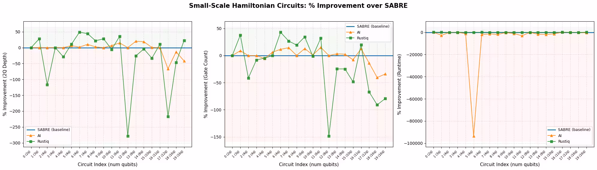
Pada skala ini, ketiga pass manager bekerja dengan baik, dan rata-rata hasilnya saling mendekati satu sama lain. Ini sebagian besar karena sirkuit kecil hanya menyisakan ruang terbatas untuk optimasi lebih lanjut, sehingga metode-metode ini cenderung menghasilkan solusi yang serupa.
Dalam contoh ini, Rustiq menghasilkan hasil yang paling bervariasi, dengan outlier terbesar dalam kedalaman dua-Qubit maupun jumlah gate. Meski variabilitas ini berarti Rustiq kadang tertinggal, ini juga berarti Rustiq kadang menemukan solusi yang lebih baik dari dua metode lainnya. Transpiler AI lebih stabil dalam hasilnya relatif terhadap SABRE dan Rustiq, mengikuti dengan dekat di sebagian besar sirkuit tanpa banyak outlier.
Untuk waktu eksekusi, SABRE dan Rustiq keduanya cepat, sedangkan transpiler bertenaga AI terlihat lebih lambat pada sirkuit-sirkuit tertentu.
Metode terbaik per metrik
Grafik di bawah menunjukkan seberapa sering setiap metode mencapai nilai terbaik (terendah) untuk setiap metrik. Seri dapat terjadi: untuk sirkuit yang lebih sederhana, beberapa metode bisa mencapai kedalaman dua-Qubit atau jumlah gate optimal yang sama. Saat seri terjadi, semua metode yang seri mendapatkan kredit, sehingga persentase untuk suatu metrik bisa berjumlah lebih dari 100%.
def plot_best_method_bars(results, metrics_list=None):
    """
    Plot a grouped bar chart showing the percentage of circuits
    where each method achieved the best (lowest) value for each metric.

    Ties are counted for all tied methods, so percentages per metric
    can sum to more than 100%.
    """
    if metrics_list is None:
        metrics_list = ["two_qubit_depth", "size", "runtime"]

    labels = {
        "two_qubit_depth": "2Q Depth",
        "size": "Gate Count",
        "runtime": "Runtime",
    }
    methods = _method_order(results)
    palette = {"SABRE": "#1f77b4", "AI": "#ff7f0e", "Rustiq": "#2ca02c"}

    by_index = {}
    for r in results:
        by_index.setdefault(r["qc_index"], []).append(r)
    n_circuits = len(by_index)

    win_data = {m: [] for m in methods}
    tie_counts = []
    metric_labels = []

    for metric in metrics_list:
        metric_labels.append(
            labels.get(metric, metric.replace("_", " ").title())
        )
        counts = Counter()
        ties = 0
        for group in by_index.values():
            min_val = min(r[metric] for r in group)
            best = [r["method"] for r in group if r[metric] == min_val]
            if len(best) > 1:
                ties += 1
            counts.update(best)
        tie_counts.append(ties)
        for m in methods:
            win_data[m].append(counts.get(m, 0) / n_circuits * 100)

    x = np.arange(len(metric_labels))
    width = 0.22
    fig, ax = plt.subplots(figsize=(8, 5))

    for i, method in enumerate(methods):
        bars = ax.bar(
            x + i * width,
            win_data[method],
            width,
            label=method,
            color=palette.get(method, None),
            edgecolor="black",
            linewidth=0.5,
        )
        for bar in bars:
            height = bar.get_height()
            if height > 0:
                ax.text(
                    bar.get_x() + bar.get_width() / 2,
                    height + 1.5,
                    f"{height:.0f}%",
                    ha="center",
                    va="bottom",
                    fontsize=9,
                )

    # Annotate tie counts below each metric label
    for j, ties in enumerate(tie_counts):
        if ties > 0:
            ax.text(
                x[j] + width,
                -8,
                f"({ties} tie{'s' if ties != 1 else ''})",
                ha="center",
                va="top",
                fontsize=8,
                color="gray",
            )

    ax.set_xticks(x + width)
    ax.set_xticklabels(metric_labels, fontsize=11)
    ax.set_ylabel("Circuits with best value (%)", fontsize=11)
    ax.set_title(
        "Best-Performing Method by Metric (ties counted for all tied methods)",
        fontsize=12,
        fontweight="bold",
    )
    ax.legend(frameon=True, fontsize=10)
    ax.set_ylim(-12, 120)
    ax.yaxis.set_major_formatter(ticker.PercentFormatter())
    ax.grid(axis="y", linestyle="--", alpha=0.4)

    plt.tight_layout()
    plt.show()
plot_best_method_bars(results_small)

Dalam contoh ini, ketiga metode berkinerja sangat mirip pada sirkuit skala kecil. Untuk kedalaman dua-Qubit dan jumlah gate, proporsi sirkuit di mana setiap metode terbaik saling berdekatan (sekitar 35–55%), dan banyak sirkuit berakhir seri karena sirkuit paling sederhana sering hanya memiliki satu solusi optimal yang ditemukan oleh beberapa metode. Perbedaan paling jelas adalah waktu eksekusi: SABRE dan Rustiq masing-masing tercepat di sekitar setengah sirkuit, sedangkan transpiler bertenaga AI jarang menjadi yang tercepat. Dengan mempertimbangkan ketiga metrik bersama, Rustiq memiliki keunggulan keseluruhan yang sedikit ia paling sering menang pada kedalaman dua-Qubit dan tetap kompetitif pada jumlah gate dan waktu eksekusi.
Langkah 3: Eksekusi menggunakan primitif Qiskit
Untuk mengevaluasi bagaimana kualitas transpilasi memengaruhi eksekusi di bawah noise, kami menggunakan teknik mirror circuit. Untuk setiap sirkuit yang ditranspilasi , kami menambahkan inversnya sehingga sirkuit gabungan secara teori adalah identitas. Mulai dari state , eksekusi sempurna (tanpa noise) akan menghasilkan bitstring all-zeros dengan probabilitas 1.
Dalam praktiknya, error gate terakumulasi di seluruh sirkuit, sehingga probabilitas mendapatkan kembali turun. Metode kompilasi yang menghasilkan sirkuit lebih dangkal dengan lebih sedikit gate akan mengakumulasi lebih sedikit noise.
Pendekatan mirror circuit ini menarik karena sederhana dan dapat diskalakan ke ukuran sirkuit apa pun, karena output yang diharapkan selalu dan tidak diperlukan simulasi klasik dari state ideal. Namun, perhatikan caveat berikut: mirror circuit adalah proksi untuk sirkuit aktual (bukan sirkuitnya sendiri), ia menggandakan jumlah gate (yang memperbesar efek noise), dan dapat meremehkan error tertentu ketika noise saling membatalkan secara simetris di sekitar batas mirror.
Kami memilih indeks sirkuit 6 dari set skala kecil dan menjalankan mirror circuit pada simulator Aer dengan model noise depolarisasi sederhana.
# Select circuit index 6 from the small-scale transpiled circuits
test_idx = 6
test_circuit = qc_small[test_idx]
print(f"Test circuit: {test_circuit.name}, {test_circuit.num_qubits} qubits")

# Get the transpiled versions
tqc_methods_small = {
    "SABRE": tqc_sabre_small[test_idx],
    "AI": tqc_ai_small[test_idx],
    "Rustiq": tqc_rustiq_small[test_idx],
}

# Show transpilation metrics for this circuit
print(f"\nTranspilation metrics for circuit index {test_idx}:")
for method, tqc in tqc_methods_small.items():
    depth_2q = tqc.depth(lambda x: x.operation.num_qubits == 2)
    size = tqc.size()
    print(f"  {method:8s}  2Q depth={depth_2q:5d}  size={size:6d}")
Test circuit: all-vib-fccf, 4 qubits

Transpilation metrics for circuit index 6:
  SABRE     2Q depth=   66  size=   339
  AI        2Q depth=   65  size=   300
  Rustiq    2Q depth=   34  size=   193
Bangun mirror circuit (tambahkan ), petakan ulang ke indeks Qubit berurutan agar simulator hanya menangani Qubit aktif, dan jalankan pada simulator Aer yang bising.
def remap_to_contiguous(tqc):
    """Remap a transpiled circuit to use contiguous qubit indices.

    Transpiled circuits target specific physical qubits (e.g., qubit 45, 67)
    on a large backend. This remaps them to 0, 1, 2, ... so Aer only
    simulates the active qubits.
    """
    active = sorted(
        {tqc.find_bit(q).index for inst in tqc.data for q in inst.qubits}
    )
    qubit_map = {old: new for new, old in enumerate(active)}
    new_qc = QuantumCircuit(len(active))
    for inst in tqc.data:
        old_indices = [tqc.find_bit(q).index for q in inst.qubits]
        new_qc.append(inst.operation, [qubit_map[i] for i in old_indices])
    return new_qc

def build_mirror_circuit(tqc):
    """Build a mirror circuit: U followed by U-dagger, with measurements.

    The combined circuit U-dagger @ U should be the identity, so measuring
    all zeros indicates a noise-free execution.
    """
    tqc_compact = remap_to_contiguous(tqc)
    mirror = tqc_compact.compose(tqc_compact.inverse())
    mirror.measure_all()
    return mirror

# Build a simple depolarizing noise model
noise_model = NoiseModel()
noise_model.add_all_qubit_quantum_error(
    depolarizing_error(0.001, 1),
    ["sx", "x", "rz"],  # ~0.1% per 1Q gate
)
noise_model.add_all_qubit_quantum_error(
    depolarizing_error(0.01, 2),
    ["cx", "ecr"],  # ~1% per 2Q gate
)

aer_sim = AerSimulator(noise_model=noise_model)

shots = 10000
fidelities = {}

for method, tqc in tqc_methods_small.items():
    mirror = build_mirror_circuit(tqc)

    sampler = SamplerV2(mode=aer_sim)
    job = sampler.run([mirror], shots=shots)
    result = job.result()
    counts = result[0].data.meas.get_counts()

    # Fidelity = fraction of all-zeros (error-free) outcomes
    n_qubits = mirror.num_qubits - mirror.num_clbits  # active qubits
    all_zeros = "0" * mirror.num_qubits
    fidelity = counts.get(all_zeros, 0) / shots
    fidelities[method] = fidelity
    print(
        f"{method:8s}  P(|00...0>) = {fidelity:.4f}  ({counts.get(all_zeros, 0)}/{shots})"
    )
SABRE     P(|00...0>) = 0.7796  (7796/10000)
AI        P(|00...0>) = 0.8073  (8073/10000)
Rustiq    P(|00...0>) = 0.8923  (8923/10000)
def plot_mirror_results(tqc_methods, fidelities, circuit_name):
    """
    Plot a three-panel comparison: fidelity, 2Q depth,
    and gate count for each compilation method.
    """
    methods = list(tqc_methods.keys())
    palette = {"SABRE": "#1f77b4", "AI": "#ff7f0e", "Rustiq": "#2ca02c"}
    colors = [palette.get(m, "gray") for m in methods]

    fidelity_vals = [fidelities[m] for m in methods]
    depth_vals = [
        tqc_methods[m].depth(lambda x: x.operation.num_qubits == 2)
        for m in methods
    ]
    size_vals = [tqc_methods[m].size() for m in methods]

    fig, axes = plt.subplots(1, 3, figsize=(16, 5))
    fig.suptitle(
        f"Mirror Circuit Results: {circuit_name}",
        fontsize=14,
        fontweight="bold",
        y=1.02,
    )

    def _annotate_bars(ax, bars, values, fmt="{}"):
        ymax = ax.get_ylim()[1]
        for bar, val in zip(bars, values):
            label = fmt.format(val)
            y = val + ymax * 0.03
            ax.text(
                bar.get_x() + bar.get_width() / 2,
                y,
                label,
                ha="center",
                va="bottom",
                fontsize=10,
                fontweight="bold",
            )

    # Panel 1: Survival Probability
    bars = axes[0].bar(
        methods, fidelity_vals, color=colors, edgecolor="black", linewidth=0.5
    )
    axes[0].set_ylabel("Fidelity  P(|00...0>)", fontsize=11)
    axes[0].set_title("Fidelity (higher is better)", fontsize=12)
    axes[0].set_ylim(
        0, max(fidelity_vals) * 1.18 if max(fidelity_vals) > 0 else 1.0
    )
    axes[0].grid(axis="y", linestyle="--", alpha=0.4)
    _annotate_bars(axes[0], bars, fidelity_vals, fmt="{:.4f}")

    # Panel 2: Two-Qubit Depth
    bars = axes[1].bar(
        methods, depth_vals, color=colors, edgecolor="black", linewidth=0.5
    )
    axes[1].set_ylabel("Two-Qubit Depth", fontsize=11)
    axes[1].set_title("2Q Depth (lower is better)", fontsize=12)
    axes[1].set_ylim(0, max(depth_vals) * 1.18)
    axes[1].grid(axis="y", linestyle="--", alpha=0.4)
    _annotate_bars(axes[1], bars, depth_vals)

    # Panel 3: Gate Count
    bars = axes[2].bar(
        methods, size_vals, color=colors, edgecolor="black", linewidth=0.5
    )
    axes[2].set_ylabel("Total Gate Count", fontsize=11)
    axes[2].set_title("Gate Count (lower is better)", fontsize=12)
    axes[2].set_ylim(0, max(size_vals) * 1.18)
    axes[2].grid(axis="y", linestyle="--", alpha=0.4)
    _annotate_bars(axes[2], bars, size_vals)

    plt.tight_layout()
    plt.show()

plot_mirror_results(tqc_methods_small, fidelities, test_circuit.name)
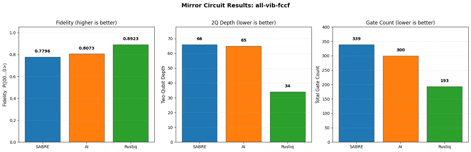
Pengamatan
Metode dengan kedalaman dua-Qubit terendah dan gate paling sedikit mencapai fidelitas tertinggi, konsisten dengan ekspektasi bahwa sirkuit yang lebih pendek mengakumulasi lebih sedikit noise. Bahkan perbedaan yang kecil dalam kedalaman dan jumlah gate menghasilkan perbedaan fidelitas yang terukur di bawah model noise depolarisasi.
Ingat bahwa hasil ini hanya untuk satu sirkuit. Peringkat relatif metode-metode ini bisa berubah dari satu sirkuit ke sirkuit lain tergantung struktur Hamiltoniannya.
Contoh perangkat keras skala besar
Di bagian ini, kami melakukan benchmark tiga metode kompilasi yang sama pada sirkuit Hamiltonian dengan 20 Qubit atau lebih. Sirkuit-sirkuit ini lebih representatif dari beban kerja simulasi Hamiltonian yang praktis dan menguji bagaimana setiap metode berkembang dalam hal kualitas sirkuit dan waktu kompilasi.
Langkah 1-4 digabungkan
Alur kerja mengikuti struktur yang sama dengan contoh skala kecil. Kami mentranspilasi semua sirkuit skala besar dengan setiap metode, mengumpulkan metrik, dan mengirimkan mirror circuit ke perangkat keras kuantum nyata.
results_large = []

tqc_sabre_large = capture_transpilation_metrics(
    results_large, pm_sabre, qc_large, "SABRE"
)
tqc_ai_large = capture_transpilation_metrics(
    results_large, pm_ai, qc_large, "AI"
)
tqc_rustiq_large = capture_transpilation_metrics(
    results_large, pm_rustiq, qc_large, "Rustiq"
)
[SABRE] Circuit 0 (all-vib-hc3h2cn): 2Q depth=2, size=258, time=0.16s
[SABRE] Circuit 1 (ham-graph-gnp_k-5): 2Q depth=345, size=4036, time=0.08s
[SABRE] Circuit 2 (TSP_Ncity-5): 2Q depth=187, size=2045, time=0.04s
[SABRE] Circuit 3 (tfim): 2Q depth=100, size=489, time=0.21s
[SABRE] Circuit 4 (all-vib-h2co): 2Q depth=30, size=570, time=0.18s
[SABRE] Circuit 5 (uuf100-ham): 2Q depth=414, size=4779, time=0.09s
[SABRE] Circuit 6 (uuf100-ham): 2Q depth=523, size=5667, time=0.11s
[SABRE] Circuit 7 (graph-gnp_k-4): 2Q depth=3028, size=24885, time=0.39s
[SABRE] Circuit 8 (uf100-ham): 2Q depth=700, size=8271, time=0.15s
[SABRE] Circuit 9 (uf100-ham): 2Q depth=698, size=8957, time=0.15s
[SABRE] Circuit 10 (TSP_Ncity-7): 2Q depth=432, size=6353, time=0.12s
[SABRE] Circuit 11 (all-vib-cyclo_propene): 2Q depth=30, size=1144, time=0.20s
[SABRE] Circuit 12 (TSP_Ncity-8): 2Q depth=704, size=10287, time=0.18s
[SABRE] Circuit 13 (uf100-ham): 2Q depth=2454, size=30195, time=0.46s
[SABRE] Circuit 14 (tfim): 2Q depth=245, size=3670, time=0.08s
[SABRE] Circuit 15 (flat100-ham): 2Q depth=154, size=3836, time=0.12s
[SABRE] Circuit 16 (graph-regular_reg-4): 2Q depth=863, size=14063, time=0.22s
[SABRE] Circuit 17 (tfim): 2Q depth=581, size=8810, time=0.15s
[SABRE] Circuit 18 (FH_D-1): 2Q depth=1704, size=9528, time=0.35s
[SABRE] Circuit 19 (TSP_Ncity-10): 2Q depth=1091, size=22041, time=0.38s
[SABRE] Circuit 20 (TSP_Ncity-10): 2Q depth=1091, size=22005, time=0.38s
[SABRE] Circuit 21 (ham-unary-color02-queen13_13_k-4): 2Q depth=224, size=8321, time=0.17s
[AI] Circuit 0 (all-vib-hc3h2cn): 2Q depth=2, size=258, time=0.17s
[AI] Circuit 1 (ham-graph-gnp_k-5): 2Q depth=323, size=4418, time=3.13s
[AI] Circuit 2 (TSP_Ncity-5): 2Q depth=161, size=2229, time=1.47s
[AI] Circuit 3 (tfim): 2Q depth=20, size=402, time=0.34s
[AI] Circuit 4 (all-vib-h2co): 2Q depth=38, size=661, time=0.19s
[AI] Circuit 5 (uuf100-ham): 2Q depth=391, size=5130, time=3.27s
[AI] Circuit 6 (uuf100-ham): 2Q depth=463, size=6095, time=4.23s
[AI] Circuit 7 (graph-gnp_k-4): 2Q depth=3207, size=25641, time=15.15s
[AI] Circuit 8 (uf100-ham): 2Q depth=637, size=8267, time=5.87s
[AI] Circuit 9 (uf100-ham): 2Q depth=632, size=9330, time=7.29s
[AI] Circuit 10 (TSP_Ncity-7): 2Q depth=452, size=7418, time=6.02s
[AI] Circuit 11 (all-vib-cyclo_propene): 2Q depth=38, size=1323, time=0.27s
[AI] Circuit 12 (TSP_Ncity-8): 2Q depth=609, size=11131, time=10.07s
[AI] Circuit 13 (uf100-ham): 2Q depth=2251, size=31128, time=38.77s
[AI] Circuit 14 (tfim): 2Q depth=165, size=3460, time=1.64s
[AI] Circuit 15 (flat100-ham): 2Q depth=91, size=3497, time=2.49s
[AI] Circuit 16 (graph-regular_reg-4): 2Q depth=664, size=15256, time=12.35s
[AI] Circuit 17 (tfim): 2Q depth=583, size=9157, time=6.28s
[AI] Circuit 18 (FH_D-1): 2Q depth=1193, size=7754, time=4.54s
[AI] Circuit 19 (TSP_Ncity-10): 2Q depth=1134, size=22577, time=25.64s
[AI] Circuit 20 (TSP_Ncity-10): 2Q depth=1172, size=23851, time=28.97s
[AI] Circuit 21 (ham-unary-color02-queen13_13_k-4): 2Q depth=219, size=8600, time=8.85s
[Rustiq] Circuit 0 (all-vib-hc3h2cn): 2Q depth=2, size=257, time=0.16s
[Rustiq] Circuit 1 (ham-graph-gnp_k-5): 2Q depth=640, size=5831, time=0.13s
[Rustiq] Circuit 2 (TSP_Ncity-5): 2Q depth=408, size=3985, time=0.08s
[Rustiq] Circuit 3 (tfim): 2Q depth=31, size=688, time=0.07s
[Rustiq] Circuit 4 (all-vib-h2co): 2Q depth=65, size=1058, time=2.91s
[Rustiq] Circuit 5 (uuf100-ham): 2Q depth=633, size=6757, time=0.14s
[Rustiq] Circuit 6 (uuf100-ham): 2Q depth=795, size=8495, time=0.17s
[Rustiq] Circuit 7 (graph-gnp_k-4): 2Q depth=13768, size=139793, time=2.92s
[Rustiq] Circuit 8 (uf100-ham): 2Q depth=1099, size=11878, time=0.25s
[Rustiq] Circuit 9 (uf100-ham): 2Q depth=911, size=11111, time=0.22s
[Rustiq] Circuit 10 (TSP_Ncity-7): 2Q depth=1183, size=13197, time=0.27s
[Rustiq] Circuit 11 (all-vib-cyclo_propene): 2Q depth=67, size=2491, time=13.56s
[Rustiq] Circuit 12 (TSP_Ncity-8): 2Q depth=1615, size=21358, time=0.48s
[Rustiq] Circuit 13 (uf100-ham): 2Q depth=2920, size=40465, time=0.91s
[Rustiq] Circuit 14 (tfim): 2Q depth=489, size=6552, time=0.15s
[Rustiq] Circuit 15 (flat100-ham): 2Q depth=378, size=5906, time=0.14s
[Rustiq] Circuit 16 (graph-regular_reg-4): 2Q depth=12163, size=168679, time=2.94s
[Rustiq] Circuit 17 (tfim): 2Q depth=1208, size=17042, time=0.36s
[Rustiq] Circuit 18 (FH_D-1): 2Q depth=1061, size=24000, time=0.47s
[Rustiq] Circuit 19 (TSP_Ncity-10): 2Q depth=2565, size=41340, time=1.38s
[Rustiq] Circuit 20 (TSP_Ncity-10): 2Q depth=2565, size=41275, time=1.38s
[Rustiq] Circuit 21 (ham-unary-color02-queen13_13_k-4): 2Q depth=808, size=17548, time=0.42s
print_summary_table(results_large)
Mean +/- std per compilation method
Method                2Q Depth              Gate Count             Runtime (s)
------------------------------------------------------------------------------
SABRE          709.1 +/- 783.8     9,100.5 +/- 8,493.1             0.2 +/- 0.1
AI             656.6 +/- 777.5     9,435.6 +/- 8,853.0            8.5 +/- 10.2
Rustiq     2,062.5 +/- 3,631.1   26,804.8 +/- 43,403.1             1.3 +/- 2.9

Mean % improvement vs SABRE (positive = better than SABRE)
Method                2Q Depth              Gate Count             Runtime (s)
------------------------------------------------------------------------------
AI             +9.6% +/- 22.8%          -3.4% +/- 9.4%    -3620.0% +/- 2405.5%
Rustiq      -154.5% +/- 273.9%      -137.1% +/- 233.2%     -527.0% +/- 1405.5%
print_per_circuit_comparison(results_large, num_rows=8)
2Q Depth (first 8 circuits by qubit count); * = best
Idx  Circuit            Q    SABRE       AI   Rustiq
----------------------------------------------------
  0  all-vib-hc3h2cn   24       2*       2*       2*
  1  ham-graph-gnp_k-  24      345     323*      640
  2  TSP_Ncity-5       25      187     161*      408
  3  tfim              26      100      20*       31
  4  all-vib-h2co      32      30*       38       65
  5  uuf100-ham        40      414     391*      633
  6  uuf100-ham        40      523     463*      795
  7  graph-gnp_k-4     40    3028*     3207    13768

Gate Count (first 8 circuits by qubit count); * = best
Idx  Circuit            Q    SABRE       AI   Rustiq
----------------------------------------------------
  0  all-vib-hc3h2cn   24      258      258     257*
  1  ham-graph-gnp_k-  24    4036*     4418     5831
  2  TSP_Ncity-5       25    2045*     2229     3985
  3  tfim              26      489     402*      688
  4  all-vib-h2co      32     570*      661     1058
  5  uuf100-ham        40    4779*     5130     6757
  6  uuf100-ham        40    5667*     6095     8495
  7  graph-gnp_k-4     40   24885*    25641   139793

Runtime (s) (first 8 circuits by qubit count); * = best
Idx  Circuit            Q    SABRE       AI   Rustiq
----------------------------------------------------
  0  all-vib-hc3h2cn   24     0.16     0.17    0.16*
  1  ham-graph-gnp_k-  24    0.08*     3.13     0.13
  2  TSP_Ncity-5       25    0.04*     1.47     0.08
  3  tfim              26     0.21     0.34    0.07*
  4  all-vib-h2co      32    0.18*     0.19     2.91
  5  uuf100-ham        40    0.09*     3.27     0.14
  6  uuf100-ham        40    0.11*     4.23     0.17
  7  graph-gnp_k-4     40    0.39*    15.15     2.92
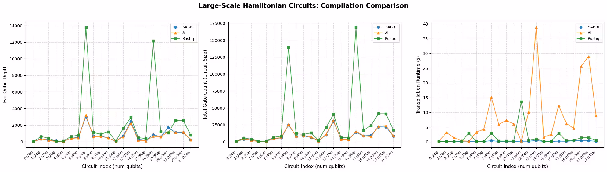
plot_transpilation_comparison(
    results_large,
    "Large-Scale Hamiltonian Circuits: Compilation Comparison",
)
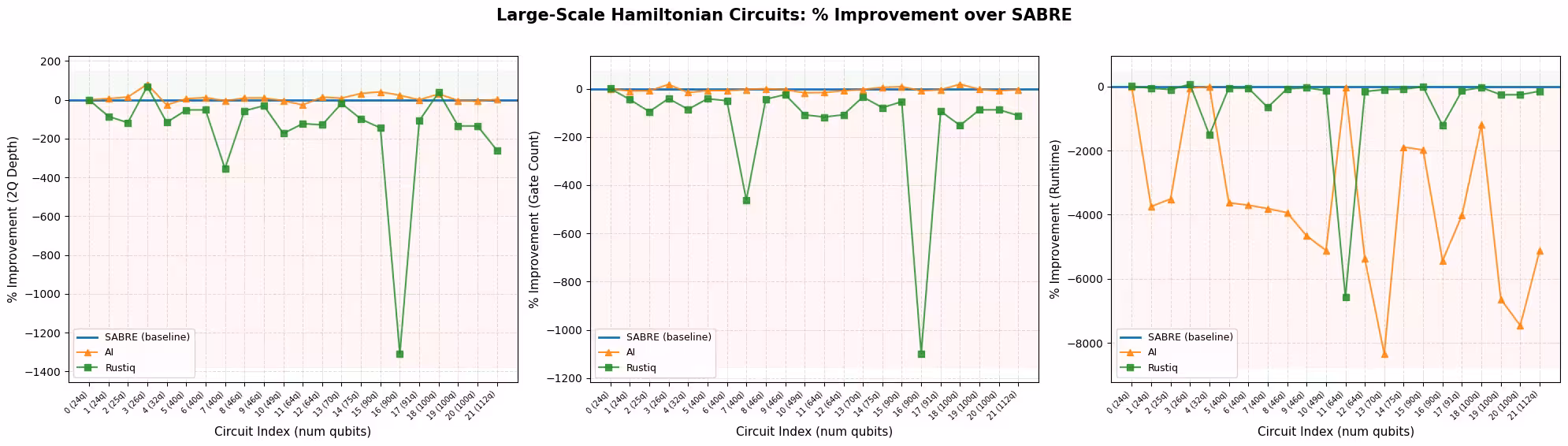
plot_pct_improvement_vs_sabre(
    results_large,
    "Large-Scale Hamiltonian Circuits",
)
plot_best_method_bars(results_large)

# Select circuit index 3 from the large-scale transpiled circuits
test_idx_large = 3
test_circuit_large = qc_large[test_idx_large]
print(
    f"Test circuit: {test_circuit_large.name}, {test_circuit_large.num_qubits} qubits"
)

tqc_methods_large = {
    "SABRE": tqc_sabre_large[test_idx_large],
    "AI": tqc_ai_large[test_idx_large],
    "Rustiq": tqc_rustiq_large[test_idx_large],
}

print(f"\nTranspilation metrics for circuit index {test_idx_large}:")
for method, tqc in tqc_methods_large.items():
    depth_2q = tqc.depth(lambda x: x.operation.num_qubits == 2)
    size = tqc.size()
    print(f"  {method:8s}  2Q depth={depth_2q:5d}  size={size:6d}")
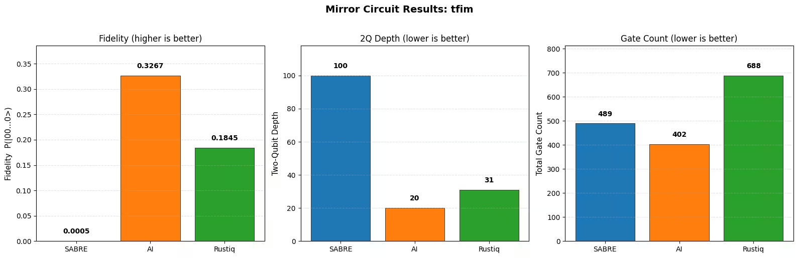
Test circuit: tfim, 26 qubits

Transpilation metrics for circuit index 3:
  SABRE     2Q depth=  100  size=   489
  AI        2Q depth=   20  size=   402
  Rustiq    2Q depth=   31  size=   688
pm_mirror = generate_preset_pass_manager(
    optimization_level=0, backend=backend
)

for method, tqc in tqc_methods_large.items():
    # print the count ops for each circuit
    mirror = tqc.copy()
    mirror.compose(tqc.inverse(), inplace=True)
    mirror.measure_all()
    mirror = pm_mirror.run(mirror)
    print(f"\n{method} transpiled circuit:")
    print(tqc.count_ops())
    print(f"{method} mirror circuit count ops:")
    print(mirror.count_ops())
SABRE transpiled circuit:
OrderedDict({'sx': 211, 'rz': 163, 'cz': 104, 'x': 11})
SABRE mirror circuit count ops:
OrderedDict({'rz': 1170, 'sx': 422, 'cz': 208, 'measure': 156, 'x': 22, 'barrier': 1})

AI transpiled circuit:
OrderedDict({'sx': 165, 'rz': 162, 'cz': 68, 'x': 7})
AI mirror circuit count ops:
OrderedDict({'rz': 984, 'sx': 330, 'measure': 156, 'cz': 136, 'x': 14, 'barrier': 1})

Rustiq transpiled circuit:
OrderedDict({'sx': 316, 'rz': 225, 'cz': 140, 'x': 7})
Rustiq mirror circuit count ops:
OrderedDict({'rz': 1714, 'sx': 632, 'cz': 280, 'measure': 156, 'x': 14, 'barrier': 1})
# Build mirror circuits and submit to real hardware
# The inverse may introduce gates (e.g., sxdg) not in the backend's
# basis gate set, so we re-transpile the mirror circuit.
pm_mirror = generate_preset_pass_manager(
    optimization_level=0, backend=backend
)

shots_hw = 10000
hw_jobs = {}

for method, tqc in tqc_methods_large.items():
    mirror = tqc.copy()
    mirror.compose(tqc.inverse(), inplace=True)
    mirror.measure_all()

    # Re-transpile at opt level 0 to decompose into basis gates
    # without changing the layout or routing
    mirror = pm_mirror.run(mirror)

    sampler = SamplerV2(mode=backend)
    sampler.options.environment.job_tags = ["TUT_CMHSC"]
    job = sampler.run([mirror], shots=shots_hw)
    hw_jobs[method] = job
    print(f"{method}: submitted job {job.job_id()}")
SABRE: submitted job d8gvgq66983c73dqe5og
AI: submitted job d8gvgqe6983c73dqe5pg
Rustiq: submitted job d8gvgqm6983c73dqe5q0
# Retrieve results and compute fidelities
fidelities_large = {}

for method, job in hw_jobs.items():
    result = job.result()
    counts = result[0].data.meas.get_counts()

    n_qubits = backend.num_qubits
    all_zeros = "0" * n_qubits
    fidelity = counts.get(all_zeros, 0) / shots_hw
    fidelities_large[method] = fidelity
    print(
        f"{method:8s}  P(|00...0>) = {fidelity:.4f}  ({counts.get(all_zeros, 0)}/{shots_hw})"
    )
SABRE     P(|00...0>) = 0.0005  (5/10000)
AI        P(|00...0>) = 0.3267  (3267/10000)
Rustiq    P(|00...0>) = 0.1845  (1845/10000)
plot_mirror_results(
    tqc_methods_large, fidelities_large, test_circuit_large.name
)
Analisis hasil kompilasi
Benchmark di atas membandingkan SABRE, transpiler bertenaga AI, dan Rustiq pada sirkuit simulasi Hamiltonian dari koleksi Hamlib pada skala kecil maupun skala besar.
Kedalaman dua-Qubit dan jumlah gate
Pada skala besar, SABRE dan transpiler bertenaga AI adalah dua performer terkuat, dan masing-masing unggul pada metrik yang berbeda. Seperti ditunjukkan grafik metode terbaik per metrik, SABRE menghasilkan jumlah gate terendah pada sebagian besar sirkuit dan merupakan metode tercepat di hampir semua sirkuit, konsisten dengan heuristik yang dirancang untuk meminimalkan gate SWAP yang disisipkan, serta optimasi terbaru pada layout dan routingnya. Transpiler bertenaga AI menghasilkan kedalaman dua-Qubit terendah pada sebagian besar sirkuit, konsisten dengan bagian tujuan reinforcement learning-nya yang menargetkan kedalaman sirkuit. Tabel ringkasan mencerminkan pembagian yang sama: SABRE memiliki rata-rata jumlah gate lebih rendah, sedangkan transpiler AI memiliki rata-rata kedalaman dua-Qubit lebih rendah. Kedua metode konsisten dan andal di seluruh rentang sirkuit.
Rustiq, yang dibangun khusus untuk sintesis PauliEvolutionGate, hanya menghasilkan hasil terbaik tunggal pada sebagian kecil sirkuit skala besar. Rata-rata metriknya sangat condong oleh beberapa outlier signifikan, terlihat sebagai lonjakan besar dalam plot perbandingan kompilasi, di mana Rustiq menghasilkan kedalaman dan jumlah gate yang jauh lebih tinggi daripada metode lainnya. Tanpa outlier ini, rata-rata performanya akan jauh lebih mendekati SABRE dan transpiler bertenaga AI.
Pengamatan utama adalah bahwa tidak ada satu metode yang mendominasi di setiap sirkuit. Setiap metode mengungguli yang lain dalam kasus tertentu, yang menjadikan worthwhile untuk mencoba semua alat yang tersedia dan memilih hasil terbaik untuk setiap sirkuit.
Waktu eksekusi
SABRE secara konsisten merupakan metode tercepat. Rustiq umumnya berjalan dengan kecepatan serupa, tetapi dapat menghasilkan outlier di mana kompilasi membutuhkan waktu jauh lebih lama. Ini terutama terlihat dalam hasil skala besar, di mana beberapa sirkuit menyebabkan waktu eksekusi Rustiq melonjak. Outlier ini sangat memengaruhi rata-rata waktu eksekusi, sehingga median mungkin merupakan ringkasan yang lebih representatif untuk Rustiq. Transpiler bertenaga AI adalah yang paling lambat dari ketiganya, dengan waktu eksekusi yang bertumbuh secara signifikan pada sirkuit yang lebih besar dan lebih kompleks.
Hasil mirror circuit
Eksperimen mirror circuit mengonfirmasi tren yang diharapkan: metode yang menghasilkan kedalaman dua-Qubit lebih rendah dan gate lebih sedikit mencapai fidelitas lebih tinggi di bawah noise. Ini berlaku baik pada simulator bising (skala kecil) maupun perangkat keras nyata (skala besar).
Ingat bahwa setiap plot mirror circuit mencerminkan satu sirkuit saja, bukan agregat. Contoh perangkat keras di atas menggunakan satu sirkuit tfim 26-Qubit, yang kebetulan merupakan kasus di mana SABRE menghasilkan kedalaman dua-Qubit yang jauh lebih tinggi daripada transpiler bertenaga AI dan Rustiq, sehingga fidelitasnya jauh lebih rendah. Ini tidak representatif dari hasil yang lebih luas: di seluruh set sirkuit skala besar, kedalaman dua-Qubit SABRE biasanya mendekati transpiler bertenaga AI, dan kedua metode masing-masing unggul pada metrik yang berbeda (transpiler bertenaga AI pada kedalaman dua-Qubit, SABRE pada jumlah gate dan waktu eksekusi). Satu hasil mirror menguji versi ganda dari satu sirkuit, bukan beban kerja penuh, sehingga tidak boleh dibaca sebagai verdict tentang kualitas metode secara keseluruhan.
Rekomendasi
Tidak ada satu strategi transpilasi terbaik untuk semua sirkuit. Pilihan terbaik bergantung pada struktur sirkuit, tujuan optimasi, dan anggaran waktu kompilasi yang tersedia:
- SABRE adalah default yang direkomendasikan. Ia cepat dan andal, serta menghasilkan hasil yang kuat di berbagai sirkuit. Untuk penyetelan lebih lanjut, pengguna dapat meningkatkan jumlah percobaan layout dan routing (lihat tutorial optimasi SABRE).
- Transpiler bertenaga AI layak dicoba ketika waktu kompilasi bukan kendala, terutama ketika minimisasi kedalaman dua-Qubit adalah prioritas: ia menghasilkan kedalaman dua-Qubit terendah pada sebagian besar sirkuit skala besar dalam benchmark ini.
- Rustiq dibangun khusus untuk sirkuit
PauliEvolutionGatedan dapat menemukan solusi berkedalaman sangat rendah dan jumlah gate rendah, terutama pada sirkuit yang lebih kecil. Pada sirkuit yang lebih besar, ia kadang menghasilkan hasil yang jauh lebih besar, sehingga paling baik digunakan sebagai salah satu dari beberapa metode yang dicoba, bukan sebagai default.
Dalam praktiknya, pendekatan terbaik adalah menjalankan semua metode yang tersedia dan memilih hasil terbaik untuk setiap sirkuit. Overhead kompilasi dari mencoba beberapa metode kecil dibandingkan dengan peningkatan potensial dalam kualitas eksekusi pada perangkat keras nyata.
Langkah selanjutnya
Jika kamu menemukan tutorial ini bermanfaat, kamu mungkin tertarik dengan hal-hal berikut:
Referensi
[1] "LightSABRE: A Lightweight and Enhanced SABRE Algorithm". H. Zou, M. Treinish, K. Hartman, A. Ivrii, J. Lishman et al. https://arxiv.org/abs/2409.08368
[2] "Practical and efficient quantum circuit synthesis and transpiling with Reinforcement Learning". D. Kremer, V. Villar, H. Paik, I. Duran, I. Faro, J. Cruz-Benito et al. https://arxiv.org/abs/2405.13196
[3] "Pauli Network Circuit Synthesis with Reinforcement Learning". A. Dubal, D. Kremer, S. Martiel, V. Villar, D. Wang, J. Cruz-Benito et al. https://arxiv.org/abs/2503.14448
[4] "Faster and shorter synthesis of Hamiltonian simulation circuits". T. Goubault de Brugiere, S. Martiel et al. https://arxiv.org/abs/2404.03280