Contoh dan aplikasi

Di pelajaran ini, kita akan menjelajahi beberapa contoh algoritma variasional dan cara menerapkannya:

• Cara menulis algoritma variasional kustom
• Cara menerapkan algoritma variasional untuk mencari nilai eigen minimum
• Cara memanfaatkan algoritma variasional untuk menyelesaikan kasus penggunaan aplikasi

Perhatikan bahwa framework pola Qiskit bisa diterapkan ke semua masalah yang kita perkenalkan di sini. Namun, untuk menghindari pengulangan, kita hanya akan menyebut langkah-langkah framework secara eksplisit dalam satu contoh kasus, yang dijalankan di hardware nyata.

Definisi masalah

Bayangkan kita ingin menggunakan algoritma variasional untuk mencari nilai eigen dari observable berikut:

$$\hat{O}_1 = 2 II - 2 XX + 3 YY - 3 ZZ,$$

Observable ini memiliki nilai eigen berikut:

$$\left\{ \begin{array}{c} \lambda_0 = -6 \\ \lambda_1 = 4 \\ \lambda_2 = 4 \\ \lambda_3 = 6 \end{array} \right\}$$

Dan eigenstate-nya:

$$\left\{ \begin{array}{c} |\phi_0\rangle = \frac{1}{\sqrt{2}}(|00\rangle + |11\rangle)\\ |\phi_1\rangle = \frac{1}{\sqrt{2}}(|00\rangle - |11\rangle)\\ |\phi_2\rangle = \frac{1}{\sqrt{2}}(|01\rangle - |10\rangle)\\ |\phi_3\rangle = \frac{1}{\sqrt{2}}(|01\rangle + |10\rangle) \end{array} \right\}$$

# Added by doQumentation — required packages for this notebook
!pip install -q numpy qiskit qiskit-ibm-runtime rustworkx scipy

from qiskit.quantum_info import SparsePauliOp

observable_1 = SparsePauliOp.from_list([("II", 2), ("XX", -2), ("YY", 3), ("ZZ", -3)])

VQE kustom

Pertama kita akan menjelajahi cara membangun instance VQE secara manual untuk mencari nilai eigen terendah dari $\hat{O}_1$. Ini akan menggabungkan berbagai teknik yang sudah kita bahas sepanjang kursus ini.

def cost_func_vqe(params, ansatz, hamiltonian, estimator):
    """Return estimate of energy from estimator

    Parameters:
        params (ndarray): Array of ansatz parameters
        ansatz (QuantumCircuit): Parameterized ansatz circuit
        hamiltonian (SparsePauliOp): Operator representation of Hamiltonian
        estimator (Estimator): Estimator primitive instance

    Returns:
        float: Energy estimate
    """
    pub = (ansatz, hamiltonian, params)
    cost = estimator.run([pub]).result()[0].data.evs

    return cost

from qiskit.circuit.library.n_local import n_local
from qiskit import QuantumCircuit

import numpy as np

reference_circuit = QuantumCircuit(2)
reference_circuit.x(0)

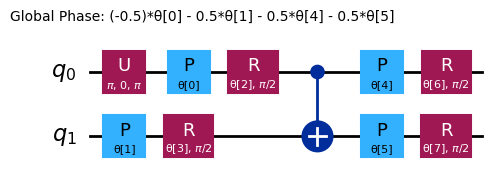
variational_form = n_local(
    num_qubits=2,
    rotation_blocks=["rz", "ry"],
    entanglement_blocks="cx",
    entanglement="linear",
    reps=1,
)

raw_ansatz = reference_circuit.compose(variational_form)
raw_ansatz.decompose().draw("mpl")

Kita akan mulai debugging di simulator lokal.

from qiskit.primitives import StatevectorEstimator as Estimator
from qiskit.primitives import StatevectorSampler as Sampler

estimator = Estimator()
sampler = Sampler()

Sekarang kita tentukan set parameter awal:

x0 = np.ones(raw_ansatz.num_parameters)
print(x0)

[1. 1. 1. 1. 1. 1. 1. 1.]

Kita bisa meminimalkan fungsi biaya ini untuk menghitung parameter optimal

# SciPy minimizer routine
from scipy.optimize import minimize
import time

start_time = time.time()

result = minimize(
    cost_func_vqe,
    x0,
    args=(raw_ansatz, observable_1, estimator),
    method="COBYLA",
    options={"maxiter": 1000, "disp": True},
)

end_time = time.time()
execution_time = end_time - start_time

Return from COBYLA because the trust region radius reaches its lower bound.
Number of function values = 103   Least value of F = -5.999999998357189
The corresponding X is:
[2.27483579e+00 8.37593091e-01 1.57080508e+00 5.82932911e-06
 2.49973063e+00 6.41884255e-01 6.33686904e-01 6.33688223e-01]

result

message: Return from COBYLA because the trust region radius reaches its lower bound.
 success: True
  status: 0
     fun: -5.999999998357189
       x: [ 2.275e+00  8.376e-01  1.571e+00  5.829e-06  2.500e+00
            6.419e-01  6.337e-01  6.337e-01]
    nfev: 103
   maxcv: 0.0

Karena masalah contoh ini hanya menggunakan dua Qubit, kita bisa memverifikasi ini dengan menggunakan solver nilai eigen aljabar linear dari NumPy.

from numpy.linalg import eigvalsh

solution_eigenvalue = min(eigvalsh(observable_1.to_matrix()))

print(f"""Number of iterations: {result.nfev}""")
print(f"""Time (s): {execution_time}""")

print(
    f"Percent error: {100*abs((result.fun - solution_eigenvalue)/solution_eigenvalue):.2e}"
)

Number of iterations: 103
Time (s): 0.4394676685333252
Percent error: 2.74e-08

Seperti yang bisa kamu lihat, hasilnya sangat dekat dengan nilai ideal.

Bereksperimen untuk meningkatkan kecepatan dan akurasi

Tambah reference state

Pada contoh sebelumnya kita tidak menggunakan operator referensi $U_R$ apapun. Sekarang mari kita pikirkan bagaimana eigenstate ideal $\frac{1}{\sqrt{2}}(|00\rangle + |11\rangle)$ bisa diperoleh. Perhatikan Circuit berikut.

from qiskit import QuantumCircuit

ideal_qc = QuantumCircuit(2)
ideal_qc.h(0)
ideal_qc.cx(0, 1)

ideal_qc.draw("mpl")

Kita bisa dengan cepat memeriksa bahwa Circuit ini memberi kita state yang diinginkan.

from qiskit.quantum_info import Statevector

Statevector(ideal_qc)

Statevector([0.70710678+0.j, 0.        +0.j, 0.        +0.j,
             0.70710678+0.j],
            dims=(2, 2))

Sekarang setelah kita melihat seperti apa Circuit yang mempersiapkan state solusi, tampaknya masuk akal untuk menggunakan Gate Hadamard sebagai Circuit referensi, sehingga ansatz lengkapnya menjadi:

reference = QuantumCircuit(2)
reference.h(0)
reference.cx(0, 1)
# Include barrier to separate reference from variational form
reference.barrier()

ref_ansatz = variational_form.decompose().compose(reference, front=True)

ref_ansatz.draw("mpl")

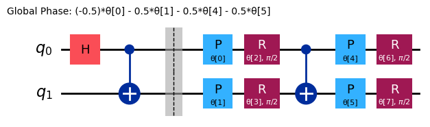
Untuk Circuit baru ini, solusi ideal bisa dicapai dengan semua parameter diset ke $0$, sehingga ini mengkonfirmasi bahwa pilihan Circuit referensi sudah masuk akal.

Sekarang mari kita bandingkan jumlah evaluasi fungsi biaya, iterasi optimizer, dan waktu yang dibutuhkan dengan percobaan sebelumnya.

import time

start_time = time.time()

ref_result = minimize(
    cost_func_vqe, x0, args=(ref_ansatz, observable_1, estimator), method="COBYLA"
)

end_time = time.time()
execution_time = end_time - start_time

Menggunakan parameter optimal kita untuk menghitung nilai eigen minimum:

experimental_min_eigenvalue_ref = cost_func_vqe(
    ref_result.x, ref_ansatz, observable_1, estimator
)
print(experimental_min_eigenvalue_ref)

-5.999999996759607

print("ADDED REFERENCE STATE:")
print(f"""Number of iterations: {ref_result.nfev}""")
print(f"""Time (s): {execution_time}""")
print(
    f"Percent error: {100*abs((experimental_min_eigenvalue_ref - solution_eigenvalue)/solution_eigenvalue):.2e}"
)

ADDED REFERENCE STATE:
Number of iterations: 127
Time (s): 0.5620882511138916
Percent error: 5.40e-08

Tergantung sistem spesifik kamu, ini mungkin atau mungkin tidak menghasilkan peningkatan kecepatan atau akurasi dalam contoh skala kecil ini. Intinya adalah bahwa memulai dengan reference state yang termotivasi secara fisik menjadi semakin penting dalam meningkatkan kecepatan dan akurasi seiring skala masalah bertambah.

Ubah titik awal

Setelah melihat efek dari penambahan reference state, kita akan melihat apa yang terjadi ketika kita memilih titik awal $\vec{\theta_0}$ yang berbeda. Secara khusus kita akan menggunakan $\vec{\theta_0}=(0,0,0,0,6,0,0,0)$ dan $\vec{\theta_0}=(6,6,6,6,6,6,6,6,6)$.

Ingat bahwa, seperti yang dibahas ketika reference state diperkenalkan, solusi ideal akan ditemukan ketika semua parameter adalah $0$, sehingga titik awal pertama seharusnya memberikan lebih sedikit evaluasi.

import time

start_time = time.time()

x0 = [0, 0, 0, 0, 6, 0, 0, 0]

x0_1_result = minimize(
    cost_func_vqe, x0, args=(raw_ansatz, observable_1, estimator), method="COBYLA"
)

end_time = time.time()
execution_time = end_time - start_time

print("INITIAL POINT 1:")
print(f"""Number of iterations: {x0_1_result.nfev}""")
print(f"""Time (s): {execution_time}""")

INITIAL POINT 1:
Number of iterations: 108
Time (s): 0.4492197036743164

Menyesuaikan titik awal ke $\vec{\theta_0}=(6,6,6,6,6,6,6,6,6)$:

import time

start_time = time.time()

x0 = 6 * np.ones(raw_ansatz.num_parameters)

x0_2_result = minimize(
    cost_func_vqe, x0, args=(raw_ansatz, observable_1, estimator), method="COBYLA"
)

end_time = time.time()
execution_time = end_time - start_time

print("INITIAL POINT 2:")
print(f"""Number of iterations: {x0_2_result.nfev}""")
print(f"""Time (s): {execution_time}""")

INITIAL POINT 2:
Number of iterations: 107
Time (s): 0.40889453887939453

Dengan bereksperimen menggunakan titik awal yang berbeda, kamu mungkin bisa mencapai konvergensi lebih cepat dan dengan lebih sedikit evaluasi fungsi.

Bereksperimen dengan optimizer yang berbeda

Kita bisa menyesuaikan optimizer menggunakan argumen method dari minimize SciPy, dengan lebih banyak opsi yang bisa ditemukan di sini. Awalnya kita menggunakan minimizer dengan batasan (COBYLA). Dalam contoh ini, kita akan menjelajahi penggunaan minimizer tanpa batasan (BFGS) sebagai gantinya

import time

start_time = time.time()

result = minimize(
    cost_func_vqe, x0, args=(raw_ansatz, observable_1, estimator), method="BFGS"
)

end_time = time.time()
execution_time = end_time - start_time

print("CHANGED TO BFGS OPTIMIZER:")
print(f"""Number of iterations: {result.nfev}""")
print(f"""Time (s): {execution_time}""")

CHANGED TO BFGS OPTIMIZER:
Number of iterations: 117
Time (s): 0.31656408309936523

Contoh VQD

Di sini kita mengimplementasikan framework Qiskit patterns secara eksplisit.

Langkah 1: Petakan input klasik ke masalah kuantum

Sekarang alih-alih hanya mencari nilai eigen terendah dari observable kita, kita akan mencari semua $4$, (di mana $k=4$).

Ingat bahwa fungsi biaya VQD adalah:

$$C_{l}(\vec{\theta}) := \langle \psi(\vec{\theta}) | \hat{H} | \psi(\vec{\theta})\rangle + \sum_{j=0}^{l-1}\beta_j |\langle \psi(\vec{\theta})| \psi(\vec{\theta^j})\rangle |^2 \quad \forall l\in\{1,\cdots,k\}=\{1,\cdots,4\}$$

Ini sangat penting karena vektor $\vec{\beta}=(\beta_0,\cdots,\beta_{k-1})$ (dalam kasus ini $(\beta_0, \beta_1, \beta_2, \beta_3)$) harus dilewatkan sebagai argumen saat kita mendefinisikan objek VQD.

Juga, dalam implementasi VQD Qiskit, alih-alih mempertimbangkan observable efektif yang dijelaskan di notebook sebelumnya, fidelitas $|\langle \psi(\vec{\theta})| \psi(\vec{\theta^j})\rangle |^2$ dihitung langsung melalui algoritma ComputeUncompute, yang memanfaatkan primitif Sampler untuk mengambil sampel probabilitas mendapatkan $|0\rangle$ untuk Circuit $U_A^\dagger(\vec{\theta})U_A(\vec{\theta^j})$. Ini berhasil karena probabilitas ini adalah

$$\begin{aligned} p_0 & = |\langle 0|U_A^\dagger(\vec{\theta})U_A(\vec{\theta^j})|0\rangle|^2 \\[1mm] & = |\big(\langle 0|U_A^\dagger(\vec{\theta})\big)\big(U_A(\vec{\theta^j})|0\rangle\big)|^2 \\[1mm] & = |\langle \psi(\vec{\theta}) |\psi(\vec{\theta^j}) \rangle|^2 \\[1mm] \end{aligned}$$

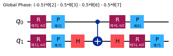
ansatz = n_local(
    num_qubits=2,
    rotation_blocks=["ry", "rz"],
    entanglement_blocks="cz",
    #    entanglement="linear",
    reps=1,
)

ansatz.decompose().draw("mpl")

Mari kita mulai dengan memeriksa observable berikut:

$$\hat{O}_2 := 2 II - 3 XX + 2 YY - 4 ZZ$$

Observable ini memiliki nilai eigen berikut:

$$\left\{ \begin{array}{c} \lambda_0 = -7 \\ \lambda_1 = 3\\ \lambda_2 = 5 \\ \lambda_3 = 7 \end{array} \right\}$$

Dan eigenstate-nya:

$$\left\{ \begin{array}{c} |\phi_0\rangle = \frac{1}{\sqrt{2}}(|00\rangle + |11\rangle)\\ |\phi_1\rangle = \frac{1}{\sqrt{2}}(|00\rangle - |11\rangle)\\ |\phi_2\rangle = \frac{1}{\sqrt{2}}(|01\rangle + |10\rangle)\\ |\phi_3\rangle = \frac{1}{\sqrt{2}}(|01\rangle - |10\rangle) \end{array} \right\}$$

from qiskit.quantum_info import SparsePauliOp

observable_2 = SparsePauliOp.from_list([("II", 2), ("XX", -3), ("YY", 2), ("ZZ", -4)])

Kita akan menggunakan fungsi berikut untuk menghitung penalti overlap. Perhatikan bahwa ini masih bagian dari pemetaan masalah ke Circuit kuantum. Namun, seperti yang dibahas di pelajaran sebelumnya, fungsi ini menghitung overlap antara Circuit variasional saat ini dan Circuit yang dioptimalkan dari state energi/biaya rendah sebelumnya yang diperoleh. Circuit baru yang dihasilkan juga harus di-transpile untuk dijalankan pada hardware nyata. Kita sudah melihat fungsi ini sebelumnya, digunakan pada simulator. Di sini, kita harus sudah mempertimbangkan transpiling dan optimisasi terkait untuk saat kita menggunakan backend nyata, oleh karena itu baris di sekitar if realbackend == 1. Ini sedikit mencampur langkah 2, tapi kita akan menyebutkan langkah 2 secara eksplisit nanti.

import numpy as np
from qiskit.transpiler.preset_passmanagers import generate_preset_pass_manager

def calculate_overlaps(
    ansatz, prev_circuits, parameters, sampler, realbackend, backend
):
    def create_fidelity_circuit(circuit_1, circuit_2):
        if len(circuit_1.clbits) > 0:
            circuit_1.remove_final_measurements()
        if len(circuit_2.clbits) > 0:
            circuit_2.remove_final_measurements()

        circuit = circuit_1.compose(circuit_2.inverse())
        circuit.measure_all()
        return circuit

    overlaps = []

    for prev_circuit in prev_circuits:
        fidelity_circuit = create_fidelity_circuit(ansatz, prev_circuit)
        if realbackend == 1:
            pm = generate_preset_pass_manager(backend=backend, optimization_level=3)
            fidelity_circuit = pm.run(fidelity_circuit)
        sampler_job = sampler.run([(fidelity_circuit, parameters)])
        meas_data = sampler_job.result()[0].data.meas

        counts_0 = meas_data.get_int_counts().get(0, 0)
        shots = meas_data.num_shots
        overlap = counts_0 / shots
        overlaps.append(overlap)

    return np.array(overlaps)

Sekarang kita tambahkan fungsi biaya VQD. Perhatikan bahwa dibandingkan pelajaran sebelumnya, kita sekarang memiliki dua argumen tambahan (realbackend dan backend) untuk membantu kita dengan transpilasi saat menggunakan backend nyata.

def cost_func_vqd(
    parameters,
    ansatz,
    prev_states,
    step,
    betas,
    estimator,
    sampler,
    hamiltonian,
    realbackend,
    backend,
):
    estimator_job = estimator.run([(ansatz, hamiltonian, [parameters])])

    total_cost = 0

    if step > 1:
        overlaps = calculate_overlaps(
            ansatz, prev_states, parameters, sampler, realbackend, backend
        )
        total_cost = np.sum(
            [np.real(betas[state] * overlap) for state, overlap in enumerate(overlaps)]
        )

    estimator_result = estimator_job.result()[0]

    value = estimator_result.data.evs[0] + total_cost

    return value

Sekali lagi, kita akan menggunakan simulator untuk debugging, lalu beralih ke hardware nyata.

from qiskit.primitives import StatevectorSampler
from qiskit.primitives import StatevectorEstimator

sampler = StatevectorSampler(default_shots=4092)
estimator = StatevectorEstimator()

Di sini kita memperkenalkan jumlah state yang ingin kita hitung, penalti, dan serangkaian parameter awal, x0.

from qiskit.quantum_info import SparsePauliOp

k = 4
betas = [50, 60, 40]
x0 = np.ones(8)

Kita sekarang akan menguji algoritma menggunakan simulator:

from scipy.optimize import minimize

prev_states = []
prev_opt_parameters = []
eigenvalues = []

realbackend = 0

for step in range(1, k + 1):
    if step > 1:
        prev_states.append(ansatz.assign_parameters(prev_opt_parameters))

    result = minimize(
        cost_func_vqd,
        x0,
        args=(
            ansatz,
            prev_states,
            step,
            betas,
            estimator,
            sampler,
            observable_2,
            realbackend,
            None,
        ),
        method="COBYLA",
        options={"maxiter": 200, "tol": 0.000001},
    )
    print(result)

    prev_opt_parameters = result.x
    eigenvalues.append(result.fun)

message: Return from COBYLA because the trust region radius reaches its lower bound.
 success: True
  status: 0
     fun: -6.9999999999996
       x: [ 1.571e+00  1.571e+00  2.519e+00  2.100e+00  1.242e+00
            6.935e-01  2.298e+00  1.991e+00]
    nfev: 151
   maxcv: 0.0
 message: Return from COBYLA because the trust region radius reaches its lower bound.
 success: True
  status: 0
     fun: 3.698974255258432
       x: [ 1.269e+00  1.109e+00  1.080e+00  1.200e+00  1.094e+00
            1.163e+00  9.752e-01  9.519e-01]
    nfev: 103
   maxcv: 0.0
 message: Return from COBYLA because the trust region radius reaches its lower bound.
 success: True
  status: 0
     fun: 4.731320121938101
       x: [ 1.533e+00  2.451e+00  2.526e+00  2.406e+00  1.968e+00
            2.105e+00  8.537e-01  8.442e-01]
    nfev: 110
   maxcv: 0.0
 message: Return from COBYLA because the trust region radius reaches its lower bound.
 success: True
  status: 0
     fun: 7.008239313655201
       x: [ 4.150e+00  2.120e+00  3.495e+00  7.262e-01  1.953e+00
           -1.982e-01  3.263e-01  2.563e+00]
    nfev: 126
   maxcv: 0.0

eigenvalues

[np.float64(-6.9999999999996),
 np.float64(3.698974255258432),
 np.float64(4.731320121938101),
 np.float64(7.008239313655201)]

Hasil ini cukup mendekati yang diharapkan kecuali untuk kesalahan aproksimasi dan fase global. Kita bisa menyesuaikan toleransi pada optimizer klasik dan/atau penalti untuk overlap statevector untuk mendapatkan nilai yang lebih presisi.

solution_eigenvalues = [-7, 3, 5, 7]

for index, experimental_eigenvalue in enumerate(eigenvalues):
    solution_eigenvalue = solution_eigenvalues[index]

    print(
        f"Percent error: {abs((experimental_eigenvalue - solution_eigenvalue)/solution_eigenvalue):.2e}"
    )

Percent error: 5.71e-14
Percent error: 2.33e-01
Percent error: 5.37e-02
Percent error: 1.18e-03

Ubah betas

Seperti yang disebutkan di pelajaran sebelumnya, nilai $\vec{\beta}$ harus lebih besar dari selisih antara nilai eigen. Mari kita lihat apa yang terjadi ketika kondisi itu tidak terpenuhi dengan $\hat{O}_2$

$$\hat{O}_2 = 2 II - 3 XX + 2 YY - 4 ZZ$$

dengan nilai eigen

$$\left\{ \begin{array}{c} \lambda_0 = -7 \\ \lambda_1 = 3\\ \lambda_2 = 5 \\ \lambda_3 = 7 \end{array} \right\}$$

from qiskit.quantum_info import SparsePauliOp

k = 4
betas = np.ones(3)
x0 = np.zeros(8)

from scipy.optimize import minimize

prev_states = []
prev_opt_parameters = []
eigenvalues = []

realbackend = 0

for step in range(1, k + 1):
    if step > 1:
        prev_states.append(ansatz.assign_parameters(prev_opt_parameters))

    result = minimize(
        cost_func_vqd,
        x0,
        args=(
            ansatz,
            prev_states,
            step,
            betas,
            estimator,
            sampler,
            observable_2,
            realbackend,
            None,
        ),
        method="COBYLA",
        options={"tol": 0.01, "maxiter": 200},
    )
    print(result)

    prev_opt_parameters = result.x
    eigenvalues.append(result.fun)

message: Return from COBYLA because the trust region radius reaches its lower bound.
 success: True
  status: 0
     fun: -6.999916534745094
       x: [ 1.568e+00 -1.569e+00  1.385e-01  1.398e-01 -7.972e-01
            7.835e-01 -2.375e-01  4.539e-02]
    nfev: 125
   maxcv: 0.0
 message: Return from COBYLA because the trust region radius reaches its lower bound.
 success: True
  status: 0
     fun: -1.515139929812874
       x: [-5.317e-04 -2.514e-03  1.016e+00  9.998e-01  3.890e-04
            1.772e-04  1.568e-04  8.497e-04]
    nfev: 35
   maxcv: 0.0
 message: Return from COBYLA because the trust region radius reaches its lower bound.
 success: True
  status: 0
     fun: -0.509948114293115
       x: [-3.796e-03  8.853e-03  3.015e-04  9.997e-01  6.271e-04
           -2.554e-03  1.017e-04  2.766e-04]
    nfev: 37
   maxcv: 0.0
 message: Return from COBYLA because the trust region radius reaches its lower bound.
 success: True
  status: 0
     fun: 0.4914672235935682
       x: [-7.178e-03 -8.652e-03  1.125e+00 -5.428e-02 -1.586e-03
            2.031e-03 -3.462e-03  5.734e-03]
    nfev: 35
   maxcv: 0.0

solution_eigenvalues = [-7, 3, 5, 7]

for index, experimental_eigenvalue in enumerate(eigenvalues):
    solution_eigenvalue = solution_eigenvalues[index]

    print(
        f"Percent error: {abs((experimental_eigenvalue - solution_eigenvalue)/solution_eigenvalue):.2e}"
    )

Percent error: 1.19e-05
Percent error: 1.51e+00
Percent error: 1.10e+00
Percent error: 9.30e-01

Kali ini, optimizer mengembalikan state yang sama $|\phi_0\rangle = \frac{1}{\sqrt{2}}(|00\rangle + |11\rangle)$ sebagai solusi yang diusulkan untuk semua eigenstate: yang jelas salah. Ini terjadi karena beta terlalu kecil untuk memberi penalti pada eigenstate minimum dalam fungsi biaya yang berurutan. Oleh karena itu, ia tidak dikecualikan dari ruang pencarian efektif pada iterasi algoritma berikutnya, dan selalu dipilih sebagai solusi terbaik yang mungkin.

Kami merekomendasikan untuk bereksperimen dengan nilai $\vec{\beta}$, dan memastikan nilainya lebih besar dari selisih antara nilai eigen.

Langkah 2: Optimalkan masalah untuk eksekusi kuantum

Untuk menjalankan ini pada hardware nyata, kita harus mengoptimalkan Circuit kuantum untuk komputer kuantum pilihan kita. Untuk tujuan di sini, kita cukup gunakan backend yang paling tidak sibuk.

from qiskit_ibm_runtime import SamplerV2 as Sampler
from qiskit_ibm_runtime import EstimatorV2 as Estimator
from qiskit_ibm_runtime import Session, EstimatorOptions
from qiskit_ibm_runtime import QiskitRuntimeService

service = QiskitRuntimeService()
backend = service.least_busy(operational=True, simulator=False)
# Or use a specific backend
# backend = service.backend("ibm_brisbane")
print(backend)

<IBMBackend('ibm_brisbane')>

Kita akan men-transpile Circuit menggunakan preset pass manager dan optimization level 3.

pm = generate_preset_pass_manager(backend=backend, optimization_level=3)
isa_ansatz = pm.run(ansatz)
isa_observable = observable_2.apply_layout(layout=isa_ansatz.layout)

Langkah 3: Eksekusi menggunakan primitif Qiskit

Dengan memastikan beta kita diatur ke nilai yang cukup tinggi, kita sekarang bisa menjalankan perhitungan pada hardware kuantum nyata.

# Estimated compute resource usage: 25 minutes. Benchmarked at 24 min, 30 sec on an Eagle r3 processor on 5-30-24

k = 2
betas = [30, 50, 80]
x0 = np.zeros(8)

real_prev_states = []
real_prev_opt_parameters = []
real_eigenvalues = []

realbackend = 1

estimator_options = EstimatorOptions(resilience_level=1, default_shots=10_000)

with Session(backend=backend) as session:
    estimator = Estimator(mode=session, options=estimator_options)
    sampler = Sampler(mode=session)

    for step in range(1, k + 1):
        if step > 1:
            real_prev_states.append(isa_ansatz.assign_parameters(prev_opt_parameters))

        result = minimize(
            cost_func_vqd,
            x0,
            args=(
                isa_ansatz,
                real_prev_states,
                step,
                betas,
                estimator,
                sampler,
                isa_observable,
                realbackend,
                backend,
            ),
            method="COBYLA",
            options={"maxiter": 200},
        )
        print(result)

        real_prev_opt_parameters = result.x
        real_eigenvalues.append(result.fun)

session.close()
print(real_eigenvalues)

Langkah 4: Post-process, kembalikan hasil dalam format klasik

Output kita secara struktural mirip dengan yang telah dibahas di pelajaran dan contoh sebelumnya. Tapi ada sesuatu yang bermasalah dalam hasil di atas, dari mana kita bisa mendapatkan pesan peringatan untuk konteks excited state. Untuk membatasi waktu komputasi yang digunakan dalam contoh pembelajaran ini, kita menetapkan jumlah iterasi maksimum untuk optimizer klasik yang mungkin terlalu rendah: 200 iterasi. Perhitungan sebelumnya di atas, pada simulator, gagal konvergen dalam 200 iterasi. Di sini, kita berhasil konvergen... tapi dengan toleransi berapa? Kita tidak menentukan toleransi agar COBYLA menganggap dirinya "konvergen". Sekilas pada nilai fungsi dan perbandingan dengan run sebelumnya memberi tahu kita bahwa COBYLA tidak mendekati konvergensi ke presisi yang kita butuhkan.

Ada masalah lain: energi excited state pertama tampaknya lebih rendah dari energi ground state! Lihat apakah kamu bisa menjelaskan bagaimana ini bisa terjadi. Petunjuk: ini berkaitan dengan titik konvergensi yang baru saja kita bahas. Perilaku ini dijelaskan secara detail di bawah setelah VQD diterapkan pada molekul H2.

Kimia kuantum: solver energi ground state dan excited state

Tujuan kita adalah meminimalkan nilai ekspektasi dari observable yang merepresentasikan energi (Hamiltonian $\hat{\mathcal{H}}$):

$$\min_{\vec\theta} \langle\psi(\vec\theta)|\hat{\mathcal{H}}|\psi(\vec\theta)\rangle$$

from qiskit.quantum_info import SparsePauliOp
from qiskit.circuit.library import efficient_su2

H2_op = SparsePauliOp.from_list(
    [
        ("II", -1.052373245772859),
        ("IZ", 0.39793742484318045),
        ("ZI", -0.39793742484318045),
        ("ZZ", -0.01128010425623538),
        ("XX", 0.18093119978423156),
    ]
)

chem_ansatz = efficient_su2(H2_op.num_qubits)

chem_ansatz.decompose().draw("mpl")

from qiskit import QuantumCircuit

def cost_func_vqe(params, ansatz, hamiltonian, estimator):
    """Return estimate of energy from estimator

    Parameters:
        params (ndarray): Array of ansatz parameters
        ansatz (QuantumCircuit): Parameterized ansatz circuit
        hamiltonian (SparsePauliOp): Operator representation of Hamiltonian
        estimator (Estimator): Estimator primitive instance

    Returns:
        float: Energy estimate
    """
    pub = (ansatz, hamiltonian, params)
    cost = estimator.run([pub]).result()[0].data.evs
    #    cost = estimator.run(ansatz, hamiltonian, parameter_values=params).result().values[0]
    return cost

Sekarang kita tetapkan serangkaian parameter awal:

import numpy as np

x0 = np.ones(chem_ansatz.num_parameters)

Kita bisa meminimalkan fungsi biaya ini untuk menghitung parameter optimal, dan kita bisa memeriksa kode kita terlebih dahulu menggunakan simulator lokal.

from qiskit.primitives import StatevectorEstimator as Estimator
from qiskit.primitives import StatevectorSampler as Sampler

estimator = Estimator()
sampler = Sampler()

# SciPy minimizer routine
from scipy.optimize import minimize
import time

start_time = time.time()

result = minimize(
    cost_func_vqe, x0, args=(chem_ansatz, H2_op, estimator), method="COBYLA"
)

end_time = time.time()
execution_time = end_time - start_time

result

message: Optimization terminated successfully.
 success: True
  status: 1
     fun: -1.857275029048451
       x: [ 7.326e-01  1.354e+00 ...  1.040e+00  1.508e+00]
    nfev: 242
   maxcv: 0.0

Nilai minimum dari fungsi biaya (-1.857...) adalah energi ground state dari molekul H2, dalam satuan hartree.

Excited States

Kita juga bisa memanfaatkan VQD untuk memecahkan $k=2$ total state (ground state dan excited state pertama).

from qiskit.quantum_info import SparsePauliOp
import numpy as np

k = 2
betas = [33, 33]
# x0 = np.zeros(ansatz.num_parameters)
x0 = [
    1.164e00,
    -2.438e-01,
    9.358e-04,
    6.745e-02,
    1.990e00,
    9.810e-02,
    6.154e-01,
    5.454e-01,
]

Kita akan tambahkan perhitungan overlap kita:

from scipy.optimize import minimize

prev_states = []
prev_opt_parameters = []
eigenvalues = []

realbackend = 0

for step in range(1, k + 1):
    if step > 1:
        prev_states.append(ansatz.assign_parameters(prev_opt_parameters))

    result = minimize(
        cost_func_vqd,
        x0,
        args=(
            ansatz,
            prev_states,
            step,
            betas,
            estimator,
            sampler,
            H2_op,
            realbackend,
            None,
        ),
        method="COBYLA",
        options={"tol": 0.001, "maxiter": 2000},
    )
    print(result)

    prev_opt_parameters = result.x
    eigenvalues.append(result.fun)

message: Optimization terminated successfully.
 success: True
  status: 1
     fun: -1.8572671093941977
       x: [ 1.164e+00 -2.437e-01  2.118e-03  6.448e-02  1.990e+00
            9.870e-02  6.167e-01  5.476e-01]
    nfev: 58
   maxcv: 0.0
 message: Optimization terminated successfully.
 success: True
  status: 1
     fun: -1.0322873777662176
       x: [ 3.205e+00  1.502e+00  1.699e+00 -1.107e-02  3.086e+00
            1.530e+00  4.445e-02  7.013e-02]
    nfev: 99
   maxcv: 0.0

eigenvalues

[-1.8572671093941977, -1.0322873777662176]

Hardware nyata dan pesan peringatan terakhir

Untuk menjalankan ini pada hardware nyata, kita harus mengoptimalkan Circuit kuantum untuk komputer kuantum pilihan kita. Untuk tujuan di sini, kita cukup gunakan backend yang paling tidak sibuk.

from qiskit_ibm_runtime import SamplerV2 as Sampler
from qiskit_ibm_runtime import EstimatorV2 as Estimator
from qiskit_ibm_runtime import Session, EstimatorOptions
from qiskit_ibm_runtime import QiskitRuntimeService

service = QiskitRuntimeService()
backend = service.least_busy(operational=True, simulator=False)

Kita akan menggunakan preset pass manager untuk transpilasi, dan kita akan memaksimalkan optimisasi Circuit menggunakan optimization level 3.

from qiskit.transpiler.preset_passmanagers import generate_preset_pass_manager

pm = generate_preset_pass_manager(backend=backend, optimization_level=3)
isa_ansatz = pm.run(ansatz)
isa_observable = H2_op.apply_layout(layout=isa_ansatz.layout)

Karena VQD sangat iteratif, kita akan menjalankan semua langkah di dalam Runtime Session, sehingga job kita hanya akan di-queue di awal, dan bukan di antara setiap pembaruan parameter. Tidak ada yang berubah dari sintaks untuk fungsi biaya atau Estimator.

x0 = [
    1.306e00,
    -2.284e-01,
    6.913e-02,
    -2.530e-02,
    1.849e00,
    7.433e-02,
    6.366e-01,
    5.600e-01,
]

# Estimated hardware usage: 20 min benchmarked on an Eagle r3 processor on 5-30-24

real_prev_states = []
real_prev_opt_parameters = []
real_eigenvalues = []

realbackend = 1

estimator_options = EstimatorOptions(resilience_level=1, default_shots=4096)

with Session(backend=backend) as session:
    estimator = Estimator(mode=session)
    sampler = Sampler(mode=session)

    for step in range(1, k + 1):
        if step > 1:
            real_prev_states.append(
                isa_ansatz.assign_parameters(real_prev_opt_parameters)
            )

        result = minimize(
            cost_func_vqd,
            x0,
            args=(
                isa_ansatz,
                real_prev_states,
                step,
                betas,
                estimator,
                sampler,
                isa_observable,
                realbackend,
                backend,
            ),
            method="COBYLA",
            options={"tol": 0.001, "maxiter": 300},
        )
        print(result)

        real_prev_opt_parameters = result.x
        real_eigenvalues.append(result.fun)

session.close()
print(real_eigenvalues)

Energi ground state yang diperoleh (-1.83 hartree) tidak terlalu jauh dari nilai yang benar (-1.85 hartree). Namun, energi excited state cukup meleset. Ini mirip dengan perilaku keliru yang kita lihat sebelumnya dalam pelajaran ini. Energi yang dilaporkan untuk excited state hampir sama dengan energi ground state. Dalam kasus sebelumnya, kita bahkan melihat energi excited state yang lebih rendah dari energi ground state yang dilaporkan.

Tidak mungkin kalkulasi variasional menghasilkan energi yang lebih rendah dari energi ground state yang sebenarnya. Dalam kasus sebelumnya, energi ground state yang kita peroleh tidak terlalu dekat dengan ground state yang sebenarnya. Karena kita tidak memperoleh energi ground state yang sebenarnya dalam kasus itu, tidak ada kontradiksi. Dalam kasus ini, energi ground state cukup dekat dengan nilai yang benar, namun energi excited state tampaknya anehnya dekat dengan nilai yang sama.

Untuk lebih memahami bagaimana ini terjadi, ingat bahwa cara kita menemukan excited state adalah dengan mensyaratkan bahwa state variasional ortogonal terhadap ground state (menggunakan overlap Circuit dan suku penalti). Jika kita gagal mendapatkan energi ground state yang akurat (atau meleset beberapa persen), maka kita juga gagal mendapatkan vektor ground state yang akurat! Jadi ketika kita mensyaratkan bahwa excited state ortogonal terhadap state pertama yang kita temukan, kita tidak memberlakukan ortogonalitas dengan ground state yang sebenarnya, melainkan dengan suatu aproksimasi dari ground state tersebut (terkadang aproksimasi yang buruk). Dengan demikian, excited state tidak dipaksa untuk ortogonal terhadap ground state yang sebenarnya, dan estimasi energi kita untuk excited state sebenarnya cukup dekat dengan energi ground state.

Ini akan selalu menjadi perhatian dalam VQD. Tapi pada prinsipnya, ini bisa dikoreksi dengan meningkatkan jumlah iterasi maksimum untuk optimizer klasik, memberlakukan toleransi lebih rendah untuk optimizer klasik, dan mungkin juga mencoba ansatz yang berbeda jika kita secara konsisten gagal menemukan ground state yang sebenarnya. Seperti yang kita lihat, seseorang mungkin juga perlu memodifikasi penalti overlap (beta). Tapi itu sebenarnya masalah yang terpisah. Tidak ada penalti untuk overlap yang akan membuat kamu menjauh dari ground state yang sebenarnya, jika kamu belum menemukan estimasi yang sangat baik dari ground state yang sebenarnya untuk overlap Circuit.

Optimasi: Max-Cut

Masalah potongan maksimum (Max-Cut) adalah masalah optimasi kombinatorial yang melibatkan pembagian simpul-simpul sebuah graf menjadi dua himpunan terpisah sehingga jumlah sisi antara kedua himpunan tersebut dimaksimalkan. Lebih formal, diberikan graf tak berarah $G=(V,E)$, di mana $V$ adalah himpunan simpul dan $E$ adalah himpunan sisi, masalah Max-Cut meminta kita untuk mempartisi simpul-simpul menjadi dua himpunan terpisah, $S$ dan $T$, sehingga jumlah sisi dengan satu titik ujung di $S$ dan titik ujung lainnya di $T$ dimaksimalkan.

Kita bisa menerapkan Max-Cut untuk menyelesaikan berbagai masalah, seperti pengelompokan, desain jaringan, dan transisi fase. Kita mulai dengan membuat graf masalah:

import rustworkx as rx
from rustworkx.visualization import mpl_draw

n = 4
G = rx.PyGraph()
G.add_nodes_from(range(n))
# The edge syntax is (start, end, weight)
edges = [(0, 1, 1.0), (0, 2, 1.0), (0, 3, 1.0), (1, 2, 1.0), (2, 3, 1.0)]
G.add_edges_from(edges)

mpl_draw(
    G, pos=rx.shell_layout(G), with_labels=True, edge_labels=str, node_color="#1192E8"
)

Masalah ini bisa diekspresikan sebagai masalah optimasi biner. Untuk setiap simpul $0 \leq i < n$, di mana $n$ adalah jumlah simpul pada graf (dalam hal ini $n=4$), kita akan mempertimbangkan variabel biner $x_i$. Variabel ini akan bernilai $1$ jika simpul $i$ berada di salah satu grup yang kita beri label $1$ dan $0$ jika berada di grup lainnya, yang kita beri label $0$. Kita juga akan menyebut $w_{ij}$ (elemen $(i,j)$ dari matriks ketetanggaan $w$) sebagai bobot sisi yang menghubungkan simpul $i$ ke simpul $j$. Karena graf tak berarah, $w_{ij}=w_{ji}$. Maka kita bisa merumuskan masalah kita sebagai memaksimalkan fungsi biaya berikut:

$$\begin{aligned} C(\vec{x}) & =\sum_{i,j=0}^n w_{ij} x_i(1-x_j)\\[1mm] & = \sum_{i,j=0}^n w_{ij} x_i - \sum_{i,j=0}^n w_{ij} x_ix_j\\[1mm] & = \sum_{i,j=0}^n w_{ij} x_i - \sum_{i=0}^n \sum_{j=0}^i 2w_{ij} x_ix_j \end{aligned}$$

Untuk menyelesaikan masalah ini dengan komputer kuantum, kita akan mengekspresikan fungsi biaya sebagai nilai ekspektasi dari sebuah observable. Namun, observable yang Qiskit dukung secara native terdiri dari operator Pauli, yang memiliki nilai eigen $1$ dan $-1$ bukan $0$ dan $1$. Itulah mengapa kita akan melakukan perubahan variabel berikut:

Di mana $\vec{x}=(x_0,x_1,\cdots ,x_{n-1})$. Kita bisa menggunakan matriks ketetanggaan $w$ untuk mengakses bobot semua sisi dengan mudah. Ini akan digunakan untuk mendapatkan fungsi biaya kita:

$$z_i = 1-2x_i \rightarrow x_i = \frac{1-z_i}{2}$$

Ini berarti bahwa:

$$\begin{array}{lcl} x_i=0 & \rightarrow & z_i=1 \\ x_i=1 & \rightarrow & z_i=-1.\end{array}$$

Sehingga fungsi biaya baru yang ingin kita maksimalkan adalah:

$$\begin{aligned} C(\vec{z}) & = \sum_{i,j=0}^n w_{ij} \bigg(\frac{1-z_i}{2}\bigg)\bigg(1-\frac{1-z_j}{2}\bigg)\\[1mm] & = \sum_{i,j=0}^n \frac{w_{ij}}{4} - \sum_{i,j=0}^n \frac{w_{ij}}{4} z_iz_j\\[1mm] & = \sum_{i=0}^n \sum_{j=0}^i \frac{w_{ij}}{2} - \sum_{i=0}^n \sum_{j=0}^i \frac{w_{ij}}{2} z_iz_j \end{aligned}$$

Selain itu, kecenderungan alami komputer kuantum adalah mencari minima (biasanya energi terendah) bukan maksima, sehingga alih-alih memaksimalkan $C(\vec{z})$ kita akan meminimalkan:

$$-C(\vec{z}) = \sum_{i=0}^n \sum_{j=0}^i \frac{w_{ij}}{2} z_iz_j - \sum_{i=0}^n \sum_{j=0}^i \frac{w_{ij}}{2}$$

Sekarang kita sudah punya fungsi biaya yang akan diminimalkan dengan variabel yang bisa bernilai $-1$ dan $1$, kita bisa membuat analogi berikut dengan Pauli $Z$:

$$z_i \equiv Z_i = \overbrace{I}^{n-1}\otimes ... \otimes \overbrace{Z}^{i} \otimes ... \otimes \overbrace{I}^{0}$$

Dengan kata lain, variabel $z_i$ akan setara dengan Gate $Z$ yang bekerja pada Qubit $i$. Selain itu:

$$Z_i|x_{n-1}\cdots x_0\rangle = z_i|x_{n-1}\cdots x_0\rangle \rightarrow \langle x_{n-1}\cdots x_0 |Z_i|x_{n-1}\cdots x_0\rangle = z_i$$

Maka observable yang akan kita pertimbangkan adalah:

$$\hat{H} = \sum_{i=0}^n \sum_{j=0}^i \frac{w_{ij}}{2} Z_iZ_j$$

yang kemudian harus kita tambahkan suku independen setelahnya:

$$\texttt{offset} = - \sum_{i=0}^n \sum_{j=0}^i \frac{w_{ij}}{2}$$

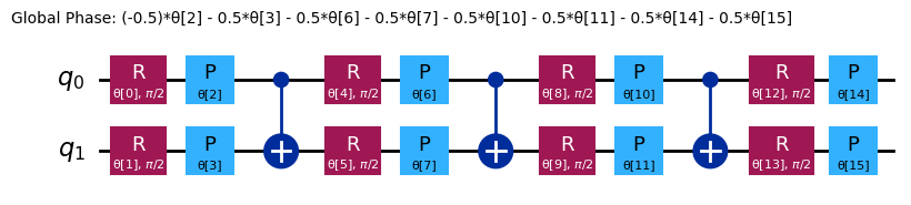
Operator ini adalah kombinasi linier dari suku-suku dengan operator Z pada simpul yang terhubung oleh sisi (ingat bahwa Qubit ke-0 ada di paling kanan): $IIZZ + IZIZ + IZZI + ZIIZ + ZZII$. Setelah operator dibuat, ansatz untuk algoritma QAOA bisa dengan mudah dibangun menggunakan Circuit QAOAAnsatz dari pustaka Circuit Qiskit.

from qiskit.circuit.library import QAOAAnsatz
from qiskit.quantum_info import SparsePauliOp

max_hamiltonian = SparsePauliOp.from_list(
    [("IIZZ", 1), ("IZIZ", 1), ("IZZI", 1), ("ZIIZ", 1), ("ZZII", 1)]
)

max_ansatz = QAOAAnsatz(max_hamiltonian, reps=2)
# Draw
max_ansatz.decompose(reps=3).draw("mpl")

# Sum the weights, and divide by 2

offset = -sum(edge[2] for edge in edges) / 2
print(f"""Offset: {offset}""")

Offset: -2.5

def cost_func(params, ansatz, hamiltonian, estimator):
    """Return estimate of energy from estimator

    Parameters:
        params (ndarray): Array of ansatz parameters
        ansatz (QuantumCircuit): Parameterized ansatz circuit
        hamiltonian (SparsePauliOp): Operator representation of Hamiltonian
        estimator (Estimator): Estimator primitive instance

    Returns:
        float: Energy estimate
    """
    pub = (ansatz, hamiltonian, params)
    cost = estimator.run([pub]).result()[0].data.evs
    #    cost = estimator.run(ansatz, hamiltonian, parameter_values=params).result().values[0]
    return cost

from qiskit.primitives import StatevectorEstimator as Estimator
from qiskit.primitives import StatevectorSampler as Sampler

estimator = Estimator()
sampler = Sampler()

Sekarang kita atur set parameter acak awal:

import numpy as np

x0 = 2 * np.pi * np.random.rand(max_ansatz.num_parameters)
print(x0)

[6.0252949  0.58448176 2.15785731 1.13646074]

Optimizer klasik apa pun bisa digunakan untuk meminimalkan fungsi biaya. Pada sistem kuantum nyata, optimizer yang dirancang untuk lanskap fungsi biaya yang tidak mulus biasanya menghasilkan hasil lebih baik. Di sini kita menggunakan rutinitas COBYLA dari SciPy melalui fungsi minimize.

Karena kita menjalankan banyak panggilan ke Runtime secara iteratif, kita menggunakan sebuah Session untuk menjalankan semua panggilan dalam satu blok. Selain itu, untuk QAOA, solusinya tersandi dalam distribusi output dari Circuit ansatz yang diikat dengan parameter optimal dari minimasi. Oleh karena itu, kita akan memerlukan primitif Sampler, dan akan menginisialisasinya dengan Session yang sama. Lalu jalankan rutinitas minimasi kita:

result = minimize(
    cost_func, x0, args=(max_ansatz, max_hamiltonian, estimator), method="COBYLA"
)

print(result)

message: Optimization terminated successfully.
 success: True
  status: 1
     fun: -2.585287311689236
       x: [ 7.332e+00  3.904e-01  2.045e+00  1.028e+00]
    nfev: 80
   maxcv: 0.0

Vektor solusi sudut parameter (x), ketika dimasukkan ke dalam Circuit ansatz, menghasilkan partisi graf yang kita cari.

eigenvalue = cost_func(result.x, max_ansatz, max_hamiltonian, estimator)
print(f"""Eigenvalue: {eigenvalue}""")
print(f"""Max-Cut Objective: {eigenvalue + offset}""")

Eigenvalue: -2.585287311689236
Max-Cut Objective: -5.085287311689235

from qiskit.result import QuasiDistribution
from qiskit.primitives import StatevectorSampler

sampler = StatevectorSampler()

# Assign solution parameters to ansatz
qc = max_ansatz.assign_parameters(result.x)

# Add measurements to our circuit
qc.measure_all()

# Sample ansatz at optimal parameters
# samp_dist = sampler.run(qc).result().quasi_dists[0]

shots = 1024
job = sampler.run([qc], shots=shots)

qc.decompose().draw("mpl")

data_pub = job.result()[0].data
bitstrings = data_pub.meas.get_bitstrings()
counts = data_pub.meas.get_counts()
quasi_dist = QuasiDistribution(
    {outcome: freq / shots for outcome, freq in counts.items()}
)
probabilities = quasi_dist

# Close the session since we are now done with it
# session.close()

from qiskit.visualization import plot_distribution

plot_distribution(counts)

binary_string = max(counts.items(), key=lambda kv: kv[1])[0]
x = np.asarray([int(y) for y in reversed(list(binary_string))])

colors = ["r" if x[i] == 0 else "c" for i in range(n)]
mpl_draw(
    G, pos=rx.shell_layout(G), with_labels=True, edge_labels=str, node_color=colors
)

Ringkasan

Dengan pelajaran ini, kamu sudah mempelajari:

• Cara menulis algoritma variasional kustom
• Cara menerapkan algoritma variasional untuk mencari nilai eigen minimum
• Cara memanfaatkan algoritma variasional untuk menyelesaikan kasus penggunaan aplikasi

Lanjut ke pelajaran terakhir untuk mengerjakan penilaianmu dan mendapatkan badge!