Mengurangi kedalaman sirkuit dengan operator backpropagation
Operator backpropagation adalah teknik yang melibatkan penyerapan operasi dari akhir sirkuit kuantum ke dalam operator Pauli, yang umumnya mengurangi kedalaman sirkuit dengan imbalan bertambahnya suku-suku dalam operator tersebut. Tujuannya adalah mem-backpropagate sebanyak mungkin bagian sirkuit tanpa membiarkan operator tumbuh terlalu besar.
Salah satu cara untuk memungkinkan backpropagation yang lebih dalam ke dalam sirkuit sekaligus mencegah operator tumbuh terlalu besar adalah dengan memotong (truncate) suku-suku dengan koefisien kecil, alih-alih menambahkannya ke operator. Pemotongan suku-suku bisa menghasilkan lebih sedikit sirkuit kuantum yang perlu dieksekusi, tapi hal ini menyebabkan sedikit kesalahan pada perhitungan nilai ekspektasi akhir yang sebanding dengan besarnya koefisien suku yang dipotong. Dalam tutorial ini kita akan mengimplementasikan sebuah pola Qiskit untuk mensimulasikan dinamika kuantum dari rantai spin Heisenberg menggunakan operator backpropagation:
- Langkah 1: Petakan ke masalah kuantum
- Petakan Hamiltonian yang berevolusi terhadap waktu ke sirkuit kuantum
- Langkah 2: Optimalkan masalah
- Iris (slice) sirkuit
- Backpropagate irisan dari sirkuit ke observable Pauli
- Gabungkan irisan yang tersisa menjadi satu sirkuit
- Transpile sirkuit untuk Backend
- Langkah 3: Jalankan eksperimen
- Hitung nilai ekspektasi menggunakan sirkuit yang diperkecil dan observable yang diperluas dengan StatevectorEstimator demi kesederhanaan dalam notebook ini
- Langkah 4: Rekonstruksi hasil
- N.A.
Catatan: Qiskit secara longgar mendefinisikan layer sebagai partisi kedalaman-1 dari sirkuit di semua qubit. Paket ini menggunakan istilah slice untuk mendeskripsikan lapisan dengan kedalaman sembarang. Fungsi qiskit_addon_obp.backpropagate dirancang untuk mem-backpropagate seluruh slice sekaligus, sehingga pilihan cara mengiris sirkuit kuantum dapat berdampak besar pada seberapa baik backpropagation bekerja untuk suatu masalah tertentu. Kamu akan mempelajari lebih lanjut tentang slice di bawah ini.
Langkah 1: Petakan ke masalah kuantum
Petakan evolusi waktu model Heisenberg kuantum ke eksperimen kuantum.
Paket qiskit_addon_utils menyediakan beberapa fungsionalitas yang dapat digunakan kembali untuk berbagai keperluan.
Modul qiskit_addon_utils.problem_generators menyediakan fungsi untuk menghasilkan Hamiltonian mirip Heisenberg pada graf konektivitas tertentu. Graf ini bisa berupa rustworkx.PyGraph atau CouplingMap sehingga mudah digunakan dalam alur kerja berbasis Qiskit.
Berikut ini, kita pertama-tama menghasilkan CouplingMap heavy-hex yang dari situ kita mengambil rantai linear 10 qubit. Perlu dicatat bahwa indeks dari reduced_coupling_map baru ini kembali berbasis nol.
# Added by doQumentation — required packages for this notebook
!pip install -q numpy qiskit qiskit-addon-obp qiskit-addon-utils qiskit-ibm-runtime rustworkx
from qiskit.transpiler import CouplingMap

coupling_map = CouplingMap.from_heavy_hex(3, bidirectional=False)

# Choose a 10-qubit linear chain on this coupling map
reduced_coupling_map = coupling_map.reduce([0, 13, 1, 14, 10, 16, 5, 12, 8, 18])
from rustworkx.visualization import graphviz_draw

graphviz_draw(reduced_coupling_map.graph, method="circo")

Selanjutnya, kita menghasilkan operator Pauli yang memodelkan Hamiltonian Heisenberg XYZ.
J_{y} \sigma_j^{y} \sigma_{k}^{y} + J_{z} \sigma_j^{z} \sigma_{k}^{z}) + \sum_{j\in V} (h_{x} \sigma_j^{x} + h_{y} \sigma_j^{y} + h_{z} \sigma_j^{z})$$ Di mana $G(V,E)$ adalah graf dari coupling map yang diberikan. ```python import numpy as np from qiskit_addon_utils.problem_generators import generate_xyz_hamiltonian # Get a qubit operator describing the Heisenberg XYZ model hamiltonian = generate_xyz_hamiltonian( reduced_coupling_map, coupling_constants=(np.pi / 8, np.pi / 4, np.pi / 2), ext_magnetic_field=(np.pi / 3, np.pi / 6, np.pi / 9), ) print(hamiltonian) ``` ```text SparsePauliOp(['IIIIIIIXXI', 'IIIIIIIYYI', 'IIIIIIIZZI', 'IIIIIXXIII', 'IIIIIYYIII', 'IIIIIZZIII', 'IIIXXIIIII', 'IIIYYIIIII', 'IIIZZIIIII', 'IXXIIIIIII', 'IYYIIIIIII', 'IZZIIIIIII', 'IIIIIIIIXX', 'IIIIIIIIYY', 'IIIIIIIIZZ', 'IIIIIIXXII', 'IIIIIIYYII', 'IIIIIIZZII', 'IIIIXXIIII', 'IIIIYYIIII', 'IIIIZZIIII', 'IIXXIIIIII', 'IIYYIIIIII', 'IIZZIIIIII', 'XXIIIIIIII', 'YYIIIIIIII', 'ZZIIIIIIII', 'IIIIIIIIIX', 'IIIIIIIIIY', 'IIIIIIIIIZ', 'IIIIIIIIXI', 'IIIIIIIIYI', 'IIIIIIIIZI', 'IIIIIIIXII', 'IIIIIIIYII', 'IIIIIIIZII', 'IIIIIIXIII', 'IIIIIIYIII', 'IIIIIIZIII', 'IIIIIXIIII', 'IIIIIYIIII', 'IIIIIZIIII', 'IIIIXIIIII', 'IIIIYIIIII', 'IIIIZIIIII', 'IIIXIIIIII', 'IIIYIIIIII', 'IIIZIIIIII', 'IIXIIIIIII', 'IIYIIIIIII', 'IIZIIIIIII', 'IXIIIIIIII', 'IYIIIIIIII', 'IZIIIIIIII', 'XIIIIIIIII', 'YIIIIIIIII', 'ZIIIIIIIII'], coeffs=[0.39269908+0.j, 0.78539816+0.j, 1.57079633+0.j, 0.39269908+0.j, 0.78539816+0.j, 1.57079633+0.j, 0.39269908+0.j, 0.78539816+0.j, 1.57079633+0.j, 0.39269908+0.j, 0.78539816+0.j, 1.57079633+0.j, 0.39269908+0.j, 0.78539816+0.j, 1.57079633+0.j, 0.39269908+0.j, 0.78539816+0.j, 1.57079633+0.j, 0.39269908+0.j, 0.78539816+0.j, 1.57079633+0.j, 0.39269908+0.j, 0.78539816+0.j, 1.57079633+0.j, 0.39269908+0.j, 0.78539816+0.j, 1.57079633+0.j, 1.04719755+0.j, 0.52359878+0.j, 0.34906585+0.j, 1.04719755+0.j, 0.52359878+0.j, 0.34906585+0.j, 1.04719755+0.j, 0.52359878+0.j, 0.34906585+0.j, 1.04719755+0.j, 0.52359878+0.j, 0.34906585+0.j, 1.04719755+0.j, 0.52359878+0.j, 0.34906585+0.j, 1.04719755+0.j, 0.52359878+0.j, 0.34906585+0.j, 1.04719755+0.j, 0.52359878+0.j, 0.34906585+0.j, 1.04719755+0.j, 0.52359878+0.j, 0.34906585+0.j, 1.04719755+0.j, 0.52359878+0.j, 0.34906585+0.j, 1.04719755+0.j, 0.52359878+0.j, 0.34906585+0.j]) ``` Dari operator qubit tersebut, kita bisa menghasilkan sirkuit kuantum yang memodelkan evolusi waktunya. Sekali lagi, modul [qiskit_addon_utils.problem_generators](https://qiskit.github.io/qiskit-addon-utils/stubs/qiskit_addon_utils.problem_generators.html) hadir dengan fungsi yang pas untuk melakukannya: ```python from qiskit.synthesis import LieTrotter from qiskit_addon_utils.problem_generators import generate_time_evolution_circuit circuit = generate_time_evolution_circuit( hamiltonian, time=0.2, synthesis=LieTrotter(reps=2), ) circuit.draw("mpl", style="iqp", scale=0.6) ``` 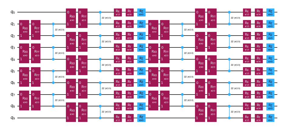 ## Langkah 2: Optimalkan masalah \{#step-2-optimize-the-problem} ### Buat irisan sirkuit untuk di-backpropagate \{#create-circuit-slices-to-backpropagate} Ingat, fungsi ``backpropagate`` akan mem-backpropagate seluruh slice sirkuit sekaligus, sehingga pilihan cara mengiris dapat berdampak pada seberapa baik backpropagation bekerja untuk suatu masalah tertentu. Di sini, kita akan mengelompokkan gate dengan tipe yang sama ke dalam slice menggunakan fungsi [slice_by_gate_types](https://qiskit.github.io/qiskit-addon-utils/stubs/qiskit_addon_utils.slicing.slice_by_gate_types.html). Untuk diskusi lebih mendetail tentang pemotongan sirkuit, lihat [panduan cara kerja](https://qiskit.github.io/qiskit-addon-utils/how_tos/create_circuit_slices.html) dari paket [qiskit-addon-utils](https://qiskit.github.io/qiskit-addon-utils/index.html). ```python from qiskit_addon_utils.slicing import slice_by_gate_types slices = slice_by_gate_types(circuit) print(f"Separated the circuit into {len(slices)} slices.") ``` ```text Separated the circuit into 18 slices. ``` ### Batasi seberapa besar operator boleh tumbuh selama backpropagation \{#constrain-how-large-the-operator-may-grow-during-backpropagation} Selama backpropagation, jumlah suku dalam operator umumnya akan mendekati $4^N$ dengan cepat, di mana $N$ adalah jumlah qubit. Ukuran operator bisa dibatasi dengan menentukan argumen kata kunci ``operator_budget`` dari fungsi ``backpropagate``, yang menerima instance [OperatorBudget](https://qiskit.github.io/qiskit-addon-obp/stubs/qiskit_addon_obp.utils.simplify.OperatorBudget.html). Di sini kita menentukan bahwa backpropagation harus berhenti ketika jumlah grup Pauli yang commuting secara qubit-wise dalam operator melebihi 8. ```python from qiskit_addon_obp.utils.simplify import OperatorBudget op_budget = OperatorBudget(max_qwc_groups=8) ``` ### Backpropagate irisan dari sirkuit \{#backpropagate-slices-from-the-circuit} Pertama, kita akan menentukan observable Pauli-Z pada qubit 0, dan kita akan mem-backpropagate irisan dari sirkuit evolusi waktu hingga suku-suku dalam observable tidak lagi bisa digabungkan menjadi 8 atau lebih sedikit grup Pauli yang commuting secara qubit-wise. Di bawah ini kamu akan melihat bahwa kita mem-backpropagate 7 slice namun hanya menggunakan 6 dari 8 grup Pauli yang dialokasikan. Ini menunjukkan bahwa mem-backpropagate satu slice lagi akan menyebabkan jumlah grup Pauli melebihi 8. Kita bisa memverifikasi hal ini dengan memeriksa metadata yang dikembalikan. ```python from qiskit.quantum_info import SparsePauliOp from qiskit_addon_obp import backpropagate from qiskit_addon_utils.slicing import combine_slices # Specify a single-qubit observable observable = SparsePauliOp("IIIIIIIIIZ") # Backpropagate slices onto the observable bp_obs, remaining_slices, metadata = backpropagate(observable, slices, operator_budget=op_budget) # Recombine the slices remaining after backpropagation bp_circuit = combine_slices(remaining_slices, include_barriers=True) print(f"Backpropagated {metadata.num_backpropagated_slices} slices.") print( f"New observable has {len(bp_obs.paulis)} terms, which can be combined into {len(bp_obs.group_commuting(qubit_wise=True))} groups." ) print( f"Note that backpropagating one more slice would result in {metadata.backpropagation_history[-1].num_paulis[0]} terms " f"across {metadata.backpropagation_history[-1].num_qwc_groups} groups." ) print("The remaining circuit after backpropagation looks as follows:") bp_circuit.draw("mpl", scale=0.6) ``` ```text Backpropagated 7 slices. New observable has 18 terms, which can be combined into 8 groups. Note that backpropagating one more slice would result in 27 terms across 12 groups. The remaining circuit after backpropagation looks as follows: ``` 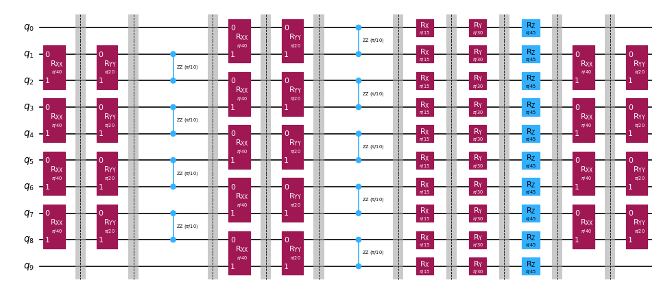 Selanjutnya, kita akan menentukan masalah yang sama dengan batasan yang sama pada ukuran observable keluaran. Namun kali ini, kita mengalokasikan anggaran error ke setiap slice menggunakan fungsi [setup_budet](https://qiskit.github.io/qiskit-addon-obp/stubs/qiskit_addon_obp.utils.truncating.setup_budget.html). Suku-suku Pauli dengan koefisien kecil akan dipotong dari setiap slice hingga anggaran error terpenuhi, dan sisa anggaran akan ditambahkan ke anggaran slice berikutnya. Untuk mengaktifkan pemotongan ini, kita perlu mengatur anggaran error seperti berikut: ```python from qiskit_addon_obp.utils.truncating import setup_budget truncation_error_budget = setup_budget(max_error_per_slice=0.005) ``` Perhatikan bahwa dengan mengalokasikan error `5e-3` per slice untuk pemotongan, kita bisa menghapus 3 slice lagi dari sirkuit, sambil tetap berada dalam anggaran awal 8 grup Pauli yang commuting dalam observable. Secara default, `backpropagate` menggunakan norma L1 dari koefisien yang dipotong untuk membatasi total error yang terjadi akibat pemotongan. Untuk opsi lainnya, lihat [panduan cara menggunakan p_norm](https://qiskit.github.io/qiskit-addon-obp/how_tos/bound_error_using_p_norm.html). Dalam contoh khusus ini di mana kita mem-backpropagate 10 slice, total error pemotongan seharusnya tidak melebihi ``(5e-3 error/slice) * (10 slices) = 5e-2``. Untuk diskusi lebih lanjut tentang mendistribusikan anggaran error di antara slice-slice kamu, lihat [panduan cara kerja ini](https://qiskit.github.io/qiskit-addon-obp/how_tos/truncate_operator_terms.html). ```python # Run the same experiment but truncate observable terms with small coefficients bp_obs_trunc, remaining_slices_trunc, metadata = backpropagate( observable, slices, operator_budget=op_budget, truncation_error_budget=truncation_error_budget ) # Recombine the slices remaining after backpropagation bp_circuit_trunc = combine_slices(remaining_slices_trunc, include_barriers=True) print(f"Backpropagated {metadata.num_backpropagated_slices} slices.") print( f"New observable has {len(bp_obs_trunc.paulis)} terms, which can be combined into {len(bp_obs_trunc.group_commuting(qubit_wise=True))} groups.\n" f"After truncation, the error in our observable is bounded by {metadata.accumulated_error(0):.3e}" ) print( f"Note that backpropagating one more slice would result in {metadata.backpropagation_history[-1].num_paulis[0]} terms " f"across {metadata.backpropagation_history[-1].num_qwc_groups} groups." ) print("The remaining circuit after backpropagation looks as follows:") bp_circuit_trunc.draw("mpl", scale=0.6) ``` ```text Backpropagated 10 slices. New observable has 19 terms, which can be combined into 8 groups. After truncation, the error in our observable is bounded by 4.933e-02 Note that backpropagating one more slice would result in 27 terms across 13 groups. The remaining circuit after backpropagation looks as follows: ```  ### Setelah mendapatkan ansatz yang diperkecil dan observable yang diperluas, kita bisa men-transpile eksperimen ke Backend. \{#now-that-we-have-our-reduced-ansatze-and-expanded-observables-we-can-transpile-our-experiments-to-the-backend} Di sini kita akan menggunakan [FakeMelbourneV2](https://quantum.cloud.ibm.com/docs/api/qiskit-ibm-runtime/fake-provider-fake-melbourne-v2) dengan 14 qubit dari [qiskit-ibm-runtime](https://quantum.cloud.ibm.com/docs/api/qiskit-ibm-runtime) untuk mendemonstrasikan cara men-transpile ke Backend QPU. ```python from qiskit.transpiler.preset_passmanagers import generate_preset_pass_manager from qiskit_ibm_runtime.fake_provider import FakeMelbourneV2 # Specify a backend and a pass manager for transpilation backend = FakeMelbourneV2() pm = generate_preset_pass_manager(backend=backend, optimization_level=1) # Transpile original experiment circuit_isa = pm.run(circuit) observable_isa = observable.apply_layout(circuit_isa.layout) # Transpile backpropagated experiment bp_circuit_isa = pm.run(bp_circuit) bp_obs_isa = bp_obs.apply_layout(bp_circuit_isa.layout) # Transpile the backpropagated experiment with truncated observable terms bp_circuit_trunc_isa = pm.run(bp_circuit_trunc) bp_obs_trunc_isa = bp_obs_trunc.apply_layout(bp_circuit_trunc_isa.layout) ``` ## Langkah 3: Jalankan eksperimen kuantum \{#step-3-execute-quantum-experiments} ### Hitung nilai ekspektasi \{#calculate-expectation-value} Akhirnya, kita bisa menjalankan eksperimen yang telah di-backpropagate dan membandingkannya dengan eksperimen penuh menggunakan [StatevectorEstimator](https://quantum.cloud.ibm.com/docs/api/qiskit/qiskit.primitives.StatevectorEstimator) yang bebas noise. Kita bisa melihat bahwa nilai ekspektasi yang di-backpropagate tanpa pemotongan setara dengan nilai eksak dalam batas presisi numerik. Nilai ekspektasi pada operator dengan suku yang dipotong memiliki sedikit error dalam orde ``1e-4``, yang masih dalam toleransi yang diharapkan. **Catatan:** Kita menggunakan primitif ``Estimator`` berbasis statevector untuk mengilustrasikan efek pemotongan pada keluaran. Untuk menjalankan pada Backend tempat eksperimen di-transpile di Langkah 2, seseorang perlu mengimpor [EstimatorV2](https://quantum.cloud.ibm.com/docs/api/qiskit-ibm-runtime/estimator-v2) dari ``qiskit-ibm-runtime`` dan memasukkan instance backend ke konstruktor. ```python from qiskit.primitives import StatevectorEstimator as Estimator estimator = Estimator() # Run the experiments using Estimator primitive result_exact = estimator.run([(circuit_isa, observable_isa)]).result()[0].data.evs.item() result_bp = estimator.run([(bp_circuit_isa, bp_obs_isa)]).result()[0].data.evs.item() result_bp_trunc = ( estimator.run([(bp_circuit_trunc_isa, bp_obs_trunc_isa)]).result()[0].data.evs.item() ) print(f"Exact expectation value: {result_exact}") print(f"Backpropagated expectation value: {result_bp}") print(f"Backpropagated expectation value with truncation: {result_bp_trunc}") print(f" - Expected Error for truncated observable: {metadata.accumulated_error(0):.3e}") print(f" - Observed Error for truncated observable: {abs(result_exact - result_bp_trunc):.3e}") ``` ```text Exact expectation value: 0.8854160687717507 Backpropagated expectation value: 0.8854160687717532 Backpropagated expectation value with truncation: 0.8850236647156059 - Expected Error for truncated observable: 4.933e-02 - Observed Error for truncated observable: 3.924e-04 ``` <TutorialFeedback />